Editing Source Node Properties
You can edit the properties of the source node by:The mixed Zoning/Surface type values are adapted from the same sources as the Agricultural and Forest source nodes
- Double clicking the left mouse button over the source node icon;
- Clicking the right mouse button on the selected source node icon and then selecting the Edit Properties menu item; or
- Pressing both the Ctrl and E keys down at the same time. The source node whose properties are to be edited must be first selected by clicking the left mouse button over the source node icon.
You will then be presented with a series of five dialogue boxes, each of which contains different parameters regarding the hydrologic and water quality characteristics of the source node.
 Tip Box
The source node property data dialogue boxes will automatically be displayed when creating a source node. The source node will only be created when the Finish button is selected on the final dialogue box
Navigating Through the Dialogue Boxes
At the bottom of each dialogue box you will find three buttons that allow you to move forward or backwards through the five dialogue boxes. You can edit any of the data presented on the active dialogue box. The buttons and their operation are described below:
| Button | Action |
|---|---|
 | Activates the next dialogue box for editing. |
 | Activates the previous dialogue box for editing. |
 | Cancels the editing session. Selecting this button on any of the dialogue boxes will terminate the editing session and all changes made to data on any of the dialogue boxes will be discarded. |
 | Ends the editing session. All changes made to the parameters displayed on any of the dialogue boxes will be accepted. The Finish button is displayed on the fifth dialogue box. |
Tip Box
When the Auto Run mode is turned on, clicking the Finish button will automatically run the simulation model. A progress bar will be displayed while the simulation is running.
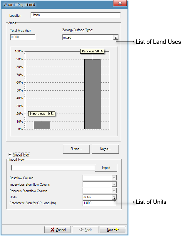
Source Node Dialogue Box, Page 1 of 5
The first dialogue box displayed contains the location name, the total area, and the proportions of impervious and pervious area for that source node. For Urban Source nodes, it also displays the zoning/surface type.
The  button allows you to record any important details or assumptions for the source node (for example, you may provide an explanation of how the impervious area was calculated).
Location
The location name will be displayed under the source node icon on the main worksheet. You may change the default location name to a more descriptive name if you wish.
Total Area
Enter the total area of this source node in hectares.
The area information forms part of the input to MUSIC’s rainfall runoff model, derived from a model developed by the CRC for Catchment Hydrology (Chiew & McMahon, 1997). For a diagram of the model structure and a brief description of its operation, see Appendix A: Rainfall-Runoff Modelling. Further guidance on setting appropriate parameters for the rainfall runoff model is contained in the Appendices, especially for parameters specific to particular regions.
Zoning/Surface Type
For Urban source nodes, select the zoning or surface type. This will change the water quality parameters used in the generation of pollutants from the source node to values appropriate for that zoning or surface type. These values are displayed on pages 3, 4 and 5 of the Wizard. See below for more details.
Pervious and Impervious Proportions
To edit the proportions of impervious and pervious areas, left click and drag the bars on the graph. The percentage value will be changed in increments of 1%.
Import Flow
This checkbox allows you to import flow time series data, resulting in the stochastic generation of constituents. Note that you must set up the pervious and impervious proportions prior to importing the time series.
Enabling this checkbox expands the dialog box so you can import the time series using the Flow Time Series Import Wizard. In the wizard, you can choose which column of the file represents various types of flow.
These are then listed in the respective fields below.
The Catchment Area for GP Loads represents the area of the catchment.
The  button allows you to save flux data (as daily or sub-daily) from the source node - such as levels in each of the soil stores, magnitudes of baseflow, throughflow and surface runoff, etc. Clicking the Fluxes button will bring up the dialogue box shown below, prompting you for a location to save the file to, and a name for the file. The text file produced can be opened in a spreadsheet, text editor, or statistics package, for further interpretation and analysis. Note that flux files can be very large.
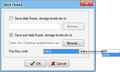
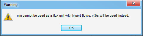
When allocating flux files and importing fluxes, ensure that Flux flow units are set up in m3/s. If you choose mm and then specify an import flux file, you will be notified of an automatic unit change with the following dialog box:
Tip Box
The time-step of the flow data and template data must be the same. If they do not match, an error will appear and you will not be able to use the time series to import flow data.
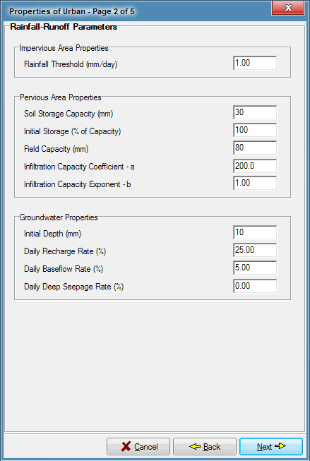
Runoff Generation Parameter Dialogue Box, Page 2 of 5
The second dialogue box displayed contains the hydrologic parameters used by the rainfall runoff model. For more information on model structure, operation and suggested parameter ranges see Rainfall Runoff Modelling. Note that if a flow time series file has been imported, these parameters will not be editable.
Impervious Area
The impervious area has depression storage only and no infiltration, and quickly produces surface runoff during an event. Water in depression storage is lost to evapotranspiration daily.
Rainfall Threshold
The rainfall threshold represents the effect of depression storage in the impervious area and defines the minimum daily rainfall (mm) before surface runoff would occur from the impervious area.
Pervious Area
The pervious area represents the fraction of the source node in which infiltration occurs. Water that is stored in the pervious storage can be lost to evapotranspiration at any time, and to groundwater when the volume in store exceeds the field capacity.
Soil Storage Capacity
Soil Storage Capacity is the maximum storage depth of the pervious area store in millimetres.
Initial Storage
Initial Storage represents the level of storage in the pervious area store at the start of the run, expressed as a percentage of the storage capacity.
Field Capacity
Field capacity is the amount of the soil capacity that, when exceeded, water in the soil stores can drain by gravity to the groundwater store. If the amount of water in the soil stores is less field capacity value, water can be removed only by evapotranspiration. Field capacity should normally be less than the soil storage capacity of the pervious store (see above).
Infiltration Capacity Coefficient (a) and Exponent (b)
These parameters are used to calculate the maximum infiltration rate into the soil store in each time interval. The maximum infiltration rate is dependent on the soil moisture level with the coefficient a defining the infiltration rate for a dry soil condition and the exponent b defining the exponential rate in which the maximum infiltration rate decreases as soil moisture level increases. Rainfall in excess of the calculated rate becomes surface runoff.
Groundwater
Groundwater is modelled as a storage beneath the pervious area, and is the only source of baseflow. Recharge is by gravity drainage from the pervious area store whenever their volume exceeds the field capacity.
Initial Depth
The Initial Depth represents the volume of groundwater at the start of the simulation, expressed as a depth in millimetres.
Daily Recharge Rate
The Daily Recharge Rate represents the amount of water that drains daily to groundwater from the soil store, expressed as a percentage of the volume above field capacity in the store.
Daily Baseflow Rate
The Daily Baseflow Rate represents the amount of water that leaves the groundwater daily as baseflow, expressed as a percentage of the current groundwater volume.
Daily Deep Seepage Rate
The Daily Deep Seepage Rate represents the amount of water that leaves the groundwater daily as seepage, expressed as a percentage of the current groundwater volume. The seepage from the groundwater store represents water that is lost from the catchment to a deep groundwater storage. This seepage is permanently lost from the model and cannot return to the catchment.
Each component of runoff is calculated using the information above and a daily time-step. Each component is then disaggregated to the required time-step, using the detailed rainfall pattern and a technique appropriate to that component. For more information on disaggregation see Appendix A: Rainfall-Runoff Modelling.
Water Quality Parameter Dialogue Boxes, Pages 3, 4 and 5 of 5
The third, fourth and fifthe dialog boxes contain the water quality parameters used in the generation of pollutants from the source node. Each dialog box is devoted to one of the pollutants modelled:
- Page 3 displays the parameters for Total Suspended Solids;
- Page 4 displays the parameters for Total Phosphorus; and
- Page 5 displays parameters for Total Nitrogen.
The pollutants are generated as concentrations in mg/L, and can be defined for both the storm flow and base flow components of runoff generated from the rainfall runoff model.
The default values displayed for Mean and Standard Deviation (Std Dev) for both base flow and storm flow (Table 1) are adapted from a range of sources, particularly Duncan (1999) and are discussed in more detail in Urban Runoff Generation. Wherever possible, these values have been modified in the MUSIC6.ini file to be representative of the region in which MUSIC is being applied.
 Tip Box
You can modify the pollutant concentrations as desired, by changing the values displayed in the Mean and Std Dev boxes. You can restore the default values of Mean and Standard Deviation for a flow component at any time by selecting the Restore Defaults button for that component. You can change the default values for these parameters in the Catchment Defaults dialog (on the Settings tab, select Defaults and then Edit).
Urban Zoning/Surface Types
For Urban source nodes, each zoning/surface type has appropriate base flow and storm flow pollutant concentrations for that zoning (eg. rural residential) or surface type (eg, sealed roads, unsealed roads). The Zoning/Surface Type is selected on Page 1 of the Wizard, and changes the default values displayed on pages 3, 4 and 5. Prior to MUSIC version 6.2, MUSIC had three source nodes, Urban, Agricultural and Forest. The 'mixed' Zoning/Surface type contains the same pollutant concentration parameters as the prior default 'Urban' values. For all other Zoning/Surface types, the pollutant concentration parameters are Sydney Catchment Authority (2012).
Table 1. Default pollutant concentrations for each source node
Source Node Type |
Zoning/Surface Type | Pollutant Concentration (log mg/L) | |||||||||||
|---|---|---|---|---|---|---|---|---|---|---|---|---|---|
| Total Suspended Solids | Total Phosphorus | Total Nitrogen | |||||||||||
| Base Flow | Storm Flow | Base Flow | Storm Flow | Base | Storm | ||||||||
| Mean | Std Dev | Mean | Std Dev | Mean | Std Dev | Mean | Std Dev | Mean | Std Dev | Mean | Std Dev | ||
| Agricultural | - | 1.40 | 0.13 | 2.30 | 0.31 | -0.88 | 0.13 | -0.27 | 0.30 | 0.074 | 0.130 | 0.59 | 0.26 |
| Forest | - | 0.90 | 0.13 | 1.90 | 0.20 | -1.50 | 0.13 | -1.10 | 0.22 | -0.14 | 0.13 | -0.075 | 0.240 |
Urban | Mixed | 1.10 | 0.17 | 2.20 | 0.32 | -8.20 | 0.19 | -0.45 | 0.25 | 0.32 | 0.12 | 0.42 | 0.19 |
| Roof | 1.10 | 0.17 | 1.30 | 0.32 | -8.20 | 0.19 | -0.89 | 0.25 | 0.32 | 0.12 | 0.30 | 0.19 | |
| Sealed Road | 1.20 | 0.17 | 2.43 | 0.32 | -8.50 | 0.19 | -0.30 | 0.25 | 0.11 | 0.12 | 0.34 | 0.19 | |
| Unsealed road | 1.20 | 0.17 | 3.00 | 0.32 | -8.50 | 0.19 | -0.30 | 0.25 | 0.11 | 0.12 | 0.34 | 0.19 | |
| Eroding gullies | 1.20 | 0.17 | 3.00 | 0.32 | -8.50 | 0.19 | -0.30 | 0.25 | 0.11 | 0.12 | 0.34 | 0.19 | |
| Revegetated land | 1.15 | 0.17 | 1.95 | 0.32 | -1.22 | 0.19 | -0.66 | 0.25 | -0.05 | 0.12 | 0.30 | 0.19 | |
| Quarries | 1.20 | 0.17 | 3.00 | 0.32 | -0.85 | 0.19 | -0.30 | 0.25 | 0.11 | 0.12 | 0.34 | 0.19 | |
| Residential | 1.20 | 0.17 | 2.15 | 0.32 | -0.85 | 0.19 | -0.60 | 0.25 | 0.11 | 0.12 | 0.30 | 0.19 | |
| Commercial | 1.20 | 0.17 | 2.15 | 0.32 | -0.85 | 0.19 | -0.60 | 0.25 | 0.11 | 0.12 | 0.30 | 0.19 | |
| Industrial | 1.20 | 0.17 | 2.15 | 0.32 | -0.85 | 0.19 | -0.60 | 0.25 | 0.11 | 0.12 | 0.30 | 0.19 | |
Rural residential | 1.15 | 0.17 | 1.95 | 0.32 | -1.22 | 0.19 | -0.66 | 0.25 | -0.05 | 0.12 | 0.30 | 0.19 | |
Tip Box
The default urban parameters were the basis for guidelines such as the Victoria Stormwater Committee (1999) BPEM Guidelines : Stormwater. It is generally recommended that these are adopted when modelling for the purposes of demonstrating compliance with this guideline. This is because using other landuse/surface types will result in larger/smaller treatment systems being required. The percentage reductions set in the guidelines combined with the 'diminishing returns' effect as concentrations decrease mean that if the starting point concentrations are lower, treatment to a percentage reduction will be harder to achieve and the required treatment size will be larger. Conversely, higher concentrations will typically require a smaller treatment system.
Tip Box
The Mean and Standard Deviation values displayed in the text boxes are displayed as the Log of the concentration in mg/L. Concentrations in the normal domain are displayed on the schematic distribution graphs on the dialogue box.
There are two options available for defining pollutant concentration in both the surface and baseflow components of the runoff:
- Mean: A constant value set at the value displayed in the Mean text box; or
- Stochastically Generated: A stochastically generated concentration whose mean and standard deviation will be consistent with those displayed in the Mean and Standard Deviation text boxes.
Tip Box
Changing the Mean and Std Dev of the Log concentrations in the text boxes will change the corresponding concentration values displayed on the accompanying graph.
When using the Stochastically generated option, the concentration at each time-step will be regenerated using a stochastic model that reproduces the mean and standard deviation of the log values displayed in the text boxes. This has been set as the default option in the model as it tends to produce a more realistic interpretation of pollutant generation from the source nodes.
A review of instantaneous water quality data has been undertaken to examine the ‘cross-correlation’ between pollutant concentrations, under both baseflow and stormflow conditions. No significant correlations were found during baseflow, however in urban catchments, a strong correlation can exist between TSS and TP during stormflow. In previous versions of music, this correlation was hard-wired, however in Version 4 and above of music, this has been removed to allow greater flexibility in the configuring of constituents.
You can specify serial correlation (autocorrelation) for both baseflow and stormflow data. The R2 for each should be derived from data in the log domain. The purpose of the stochastic generation option is to provide more realistic temporal variations in concentration; in other words, the concentration predicted by music at time t will be related to (correlated with) the concentration at the previous time-step (t-1). This results in pollutographs (plots of pollutant concentration over time) which are more realistic.
The default autocorrelation coefficient is set to zero to allow the same model run by different users to produce the same magnitude of loads, however you can specify the auto correlation coefficient if required (say if needing to calibrate against measured concentration data) and should use the values as set out in the table below:
| Time-step | Autocorrelation coefficient | |
|---|---|---|
| Baseflow | Stormflow | |
| 6-min | 0.94 | 0.95 |
| 12-min | 0.82 | 0.93 |
| 30-min | 0.51 | 0.84 |
| 1-hour | 0.41 | 0.77 |
| 3-hour | 0.37 | 0.62 |
| 6-hour | 0.35 | 0.50 |
| Day | 0.31 | 0.27 |
It is important to note that the autocorrelation coefficient will not significantly affect the treatment train effectiveness produced by music, but simply ensures that the variation over time in concentrations during storm events and baseflow conditions is more ‘realistic’. Depending on the time-step and coefficient used, there can be variations in mean annual loads for the same model run on different computers, however the maximum difference is usually within 10% of the previous run.
Tip Box
Serial correlation (also called autocorrelation) is the correlation between pollutant concentration at time t, and the previous time-step, t-1. music does not model autocorrelation for lag periods of more than one time-step.