| Info | ||
|---|---|---|
| ||
Some features are not available in Source (public version). |
Introduction
...
- First, create a schematic scenario;
- Choose Tools » River Operations to open the River Operations dialog (Figure 1); and
- Click on the slider below Operations Mode to ON.
Once you have created forecast models, you can disable operations, but retain these models or overrides using the buttons under Operations Data. The first two buttons in this dialog deal with removing input data, whereas the third one deletes all output data that was created for the forecast models. To clear all operations related data (input, output as a well as overrides), click Clear ALL Operations Data.
Figure 1. River Operations
...
The Constituents tab gets enabled when constituents have been configured in a scenario (its operation is similar to the Constituents tab in a single analysis run).
| Anchor | ||||
|---|---|---|---|---|
|
...
Figure 4. Inflow node, Operations forecasting
Figure 5. Storage Routing Link, Operations forecasting
| Info | ||
|---|---|---|
| ||
| Note: Forecast scenarios are unique to a node and must be configured individually for each node. |
...
Forecast model type | Description |
|---|---|
| Average | Allows you to define the average over the last specified number of time-steps. |
Function | Allows you to define a function to return any value you choose for each time-step in the forecast period. For example:
|
Monthly Average | Allows you to enter an average forecast value, in megalitres per day, to be applied for the whole of each month. You can either enter the monthly average values manually, or import the values from a .CSV file formatted as shown in Table 2. To trend from "today" to the monthly average, enable the Trend to Value at Rate checkbox and enter a trend rate which is a real number greater than zero but less than one. The observed daily flow rate for the previous month and the number of days of the current month are used to determine the initial flow volume. |
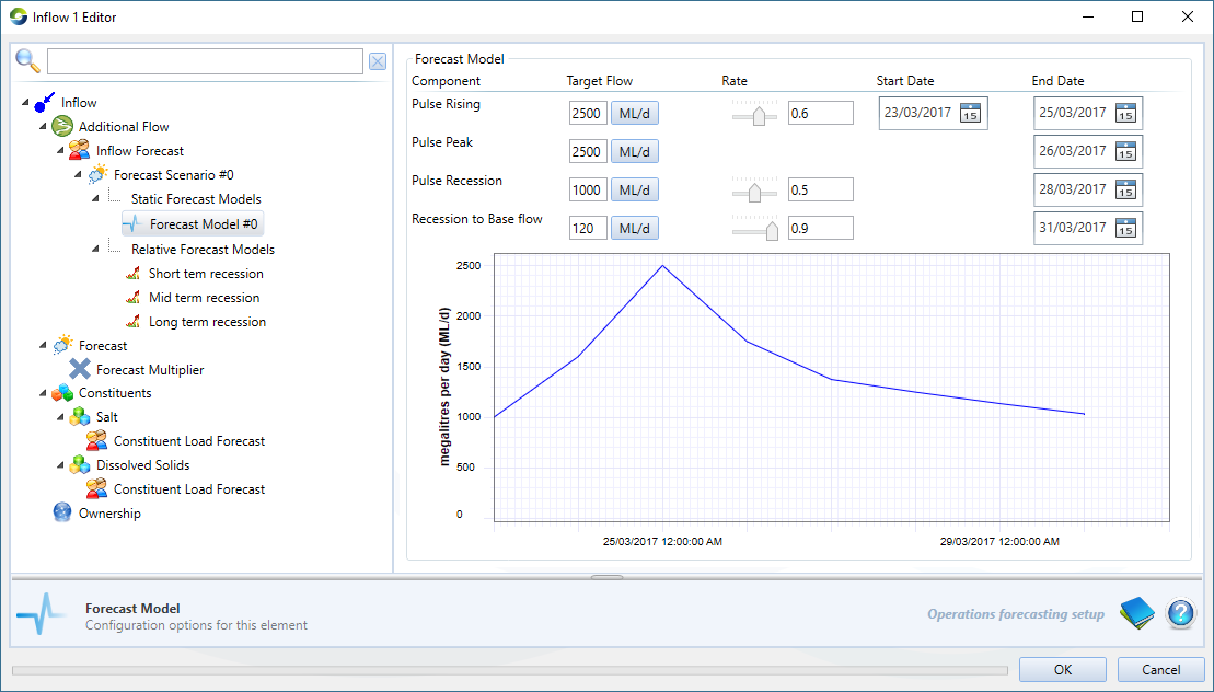
| Pulse | Allows a static forecast model that is applied on a specified date and has priority over other relative forecast models if enabled. The forecast pulse flow rate is entered under the Target Flow configuration, and the pulse start and end dates are specified with the date inputs. The rate of the rise and recession of the pulse is configured by the Rate sliders or can be entered directly as value. For example, the 0.6 Rate of the Pulse Rising indicates that at each time step there is an increase of 60% in the flow volume until the Target Flow is reached.. |
Time Series | To specify a forecast based on a time series, you must:
Time series are assumed to conform with the structure shown in Table 3. Note that any time-stamps contained in a time series are ignored. The observation in the first row of the time series is used for the first time-step of the forecast period, the observation in the second row for the second time-step, and so on, until either there are no more data rows in the time series or the simulation reaches the end of the forecast period. |
Trend | A single target value (either positive or negative) plus a recession rate. To specify a trend forecast, enter the target value in megalitres per day, and use the slider to specify the trend rate, which is a real number greater than zero but less than one. |
Figure 6. Pulse Forecast Model
Table 2. Monthly average forecasting model (data file format)
...
