Appendix A: Rainfall-Runoff Modelling
Introduction
The algorithm adopted to generate urban runoff is based on a simplified rainfall-runoff model developed by Chiew et al. (1997). The model was initially developed using a daily timestep, but has been modified for incorporation into MUSIC to allow disaggregation of the generated daily runoff into sub-daily temporal patterns.
Description Of Daily Rainfall-Runoff Model
The structure of the rainfall-runoff model and the conceptual representation of the processes involved are shown in Figure 1. The model allows for separate runoff generation processes on impervious and pervious portions of a catchment.
All rainfall on the impervious area becomes runoff once a small storage capacity or initial loss is exceeded. The initial loss storage is emptied each day.
In MUSIC Version 2, pervious areas are modelled using one soil moisture store and one groundwater store, as shown in Figure 1. The two parallel soil moisture stores of MUSIC Version 1 have been reduced to one, since there is rarely enough observed data to calibrate the additional store.
Rainfall on the pervious part of the catchment is subject to infiltration, with the infiltration rate of the soil being defined as an exponential function of the soil moisture storage. The infiltration rate is at a maximum when the soil moisture store is empty, and gradually decreases to a minimum when the soil moisture store is full. Runoff from the pervious area occurs when the rainfall exceeds the infiltration rate of the soil (infiltration excess runoff) and when the soil moisture store has reached its maximum capacity (soil saturation excess runoff).
Evapotranspiration is subtracted from the soil moisture store. It is dependant on the amount of water in the soil store and the areal potential evapotranspiration rate.
Soil moisture recharges groundwater whenever the soil moisture store exceeds field capacity. Recharge is calculated as a constant percentage of the storage above field capacity. Baseflow from groundwater is simulated using a linear recession of the groundwater store.

Figure 1: Conceptual daily rainfall-runoff model adopted for MUSIC.
Disaggregation Of Modelled Daily Runoff Into Sub-Daily Time Steps
An approximate daily runoff disaggregating procedure has been adopted to define sub-daily temporal patterns for the modelled daily runoff totals. The pervious and impervious areas are treated separately. The computational steps in the disaggregating procedure are described below.
Impervious area runoff
The daily model assumes an empty impervious store at the start of each day. The rainfall from the initial time steps is subtracted until the impervious store (initial loss) is satisfied. The remaining rainfall in the sub-daily distribution is taken to be the runoff time series from the impervious area. The resulting rainfall excess temporal pattern is illustrated in Figure 2.
Pervious area surface runoff
The pervious area surface runoff distribution is derived from the sub-daily temporal pattern of rainfall by satisfying infiltration excess runoff, evaporation losses, soil moisture storage deficit and saturation excess runoff in order.
The temporal distribution of infiltration excess runoff is represented by the rainfall temporal pattern during the period of infiltration excess rainfall conditions. The daily evaporation loss is then removed from the temporal pattern uniformly over the duration of the storm, followed by the soil moisture deficit. The soil moisture deficit is subtracted from the early periods of the rainfall temporal pattern to reflect the progressive increase in soil moisture, leading ultimately to the occurrence of soil saturation excess runoff. The residual rainfall temporal pattern after accounting for the soil moisture deficit corresponds to the saturation excess runoff distribution. The disaggregation procedure is illustrated in Figure 2.

Figure 2: Disaggregation of daily runoff into sub-daily temporal patterns
Disaggregated Runoff Time Series
The daily baseflow total is uniformly distributed over the sub-daily time steps. The temporal pattern of the total runoff from the catchment is the combined time series of the impervious runoff, infiltration excess runoff, saturation excess runoff and baseflow patterns.
Calibration
The rainfall runoff model should be calibrated to local conditions whenever possible, using any available data from within or near the catchment. The default values have not been calibrated to your catchment. It is recognised that there will rarely be sufficient data in practice to fully calibrate every model parameter. But even a partial calibration will lead to greatly improved results. The following suggestions may assist with the calibration process.
Mean Rainfall
If the mean catchment rainfall is known to be slightly different from that at the rain gauge being used (e.g. from isohyetal maps), an approximate but effective adjustment can be applied by changing the total catchment area. For example, if mean catchment rainfall is 15% higher than at the rain gauge site, increase the catchment area by 15%. If the catchment rainfall is very different from that at the rain gauge, it is likely that the temporal pattern is also very different. A more representative rain gauge will give better results.
Runoff Volume
If the actual runoff volume over a period is known, the simulated runoff volume can be made to match by adjusting the modelled impervious percentage and/or the deep seepage rate. Simulated annual runoff at any node is tabulated in the Statistics / Mean Annual Loads information box for that node. Rainfall on impervious areas quickly becomes runoff (except for a small initial loss in depression storage), but rainfall on pervious areas is subject to losses by evapotranspiration from the soil store and deep seepage from the groundwater store.
The impervious percentage for an urban catchment will typically be closer to the directly connected impervious area than the total impervious area.
The deep seepage rate can vary considerably, depending on geology and soil type. In a given area it will typically be highest for small first order (upstream) catchments, less for larger first order catchments, and close to zero for incremental catchment areas further downstream. This just reflects the observation that small upstream catchments typically produce less baseflow per unit area than larger downstream catchments do.
Flow Data
Calibration to observed flow data is best carried out by importing the observed data into MUSIC. Observed data at any node can be imported using the Observed Data / Import... dialogue box for that node. Spreadsheet programs such as Excel can save data in the required csv (comma separated variable) format. Imported data can be displayed together with simulated behaviour in time series graphs for that node (and can be turned off when not needed using the Edit Graph Properties button).
Baseflow
All baseflow is derived from the groundwater store, which is recharged in turn from the pervious soil store. Adjust the daily drainage rate, then the daily recharge rate, then the pervious soil storage capacity if necessary, to improve the fit between simulated and observed baseflow.
If the warm-up feature is enabled, MUSIC estimates initial storage levels by running one year of data before starting the full simulation. In this case the initial groundwater depth and the initial pervious soil storage should be reasonable, but are unlikely to be the values entered in the node setup. If the warm-up is not used, adjust the initial groundwater depth and the initial pervious soil storage, if necessary, to improve the fit in the early part of the record.
Stormflow
Stormflow is generated principally from the impervious area, and under some conditions from the pervious area as well. Increase the fraction impervious to increase the stormflow volume.
If sufficient information is available, simulated stormflow can be further modified by changing the pervious soil storage capacity and/or the infiltration parameters. Reducing the pervious soil storage capacity will increase the stormflow generated by soil saturation. Soil capacity should not normally be less than field capacity. Reducing the maximum infiltration rate (coefficient a) will increase the stormflow generated when rainfall cannot infiltrate fast enough.
Check Flow Volumes
If significant changes have been made to the model parameters during the calibration process, it will be necessary to go back and check the total flow volumes again. Changes to the infiltration and soil store parameters affect the volume of water lost by evapotranspiration and deep seepage, and so affect the whole water balance of the catchment. For this reason an iterative approach is required.
Default Parameters
The rainfall-runoff model should be calibrated to local conditions whenever possible. Based on information available to date, the following values could serve as a starting point for the calibration process. Remember that MUSIC can estimate the two initial capacities for a given run by using the warm-up option, provided the run duration is twelve months or more.
Impervious threshold | 1 mm |
|---|---|
Initial soil storage | 30% |
Infiltration capacity | 200 mm |
Infiltration exponent | 1 |
Initial groundwater store | 10 mm |
Daily recharge rate | 25% |
Daily drainage rate | 5% |
Daily deep seepage rate | 0% |
The following parameters are more dependent on location.
Location | Soil Store Capacity (mm) | Field Capacity (mm) |
|---|---|---|
Darwin | 300 | 250 |
Brisbane | 120 | 80 |
Sydney | 200 | 170 |
Canberra | 40 | 25 |
Melbourne | 30 | 20 |
Hobart | 30 | 20 |
Adelaide | 40 | 30 |
Perth | 250 | 230 |
The rainfall-runoff model should be calibrated to local conditions whenever possible.
For application in the UK, the MUSIC hydrologic model has been compared to similar UK hydrologic models and methods, in addition to calibration of the model to gauged data for several catchments to assist in deriving suitable parameters.
Similarities to UK Models
There are numerous similarities to existing UK hydrological models. The closest similarity is to the PDM conceptualisation. Fixing values of certain parameters within the PDM model and by making the surface and groundwater stores linear it is possible to almost replicate the response of the pervious fraction of the MUSIC model. The differences are that PDM does not allow for infiltration excess overland flow as it is not perceived to be as commonly observed as saturation excess overland flow in the UK.
As the ReFH model utilises the same soil stores as the PDM model it also shares many similarities with MUSIC, with the added advantage that regression formulae exist for estimating a number of the key parameters.
The key difference in application between the MUSIC hydrological model and existing UK models is that it requires some form of routing to be undertaken on the overland flow in order to replicate observed flows at the event scales whilst both PDM and ReFH have runoff routing functions in built.
It should be clarified that the hydrological model in MUSIC was built for different purposes to both PDM and ReFH which are intended as flood forecasting and flood estimation tools respectively.
The Wallingford Procedure is the primary method for calculating runoff in urban catchments within the UK, although revisions such as the ‘New UK Runoff Model’ have been proposed since its inception.
Another model that has been commonly used in the UK at various times is HYSIM. HYSIM is a hydrological simulation model which uses rainfall and potential evaporation data to simulate the hydrological cycle (surface runoff, percolation to groundwater and river flow) on a continuous basis. Overall the model is similar to the hydrological model in MUSIC, however the model structure is less conceptual and based more on the physical processes. There are a number of soil store layers within HYSIM rather than the two within MUSIC.
This would allow HYSIM to better represent the physical processes but in the absence of observed data the additional parameters make it difficult to calibrate.
Parameterisation of the MUSIC rainfall runoff model in the UK
The majority of the MUSIC parameters can be replicated from existing UK models or literature, a description of this process is given below:
1. Impervious threshold
This is analogous to the depression storage term used in the Wallingford procedure. Depression storage (DS) is calculated from the overland slope (in %) of the catchment using the formula:
DS = 0.71SLOPE-0.48
and the suggestion that for pitched roofs DS should be equal to 0.4mm.
2. Initial Soil Storage
Ideally this should be calibrated from observed data where available but ReFH offers a means for estimating seasonal values based on FEH catchment descriptors:
Cini (Winter) = 298.35BFIHOST0.95PROPWET-0.24(1.20-1.70BFIHOST+0.82PROPWET)
Cini (Summer) = 298.35BFIHOST0.95PROPWET-0.24(0.90-0.82BFIHOST-0.43PROPWET)
It should be noted that these estimators are based on a very small sample set of observed events (Winter, n = 93; Summer, n = 7) and the fit to them is not wonderful (Winter, r2 = 0.53; Summer, r2 = 0.49). The values could also be negative in which case they are set to 0.
3. Infiltration Capacity
Generally UK models do not consider infiltration excess to be the dominant process in runoff generation and it is not usually physically represented as rainfall intensity rarely exceeds infiltration capacity. For parameterisation purposes this could be set to a sufficiently high value that rainfall will not exceed infiltration or it could be parameterised using literature values (possibly referring back to the HOST soils classification).
4. Infiltration Exponent
This will likely remain as the Australian default value of 1 in the absence of any literature proposing a more suitable value.
5. Initial Groundwater Storage
As with the initial soil storage this can and should be calibrated from observed data when available by using the warm up function. The groundwater store in MUSIC differs to that of the FEH Methods which do not include an explicit store. The PDM does have an explicit store but there are no obvious literature values for calibrating it to.
6. Daily recharge rate
The ReFH model use a daily recharge rate, k defined as:
DK=exp(-kΔt)=0.8 which yields k=0.223
This compares favourably with the MUSIC default of 25%.
7. Daily drainage rate
There is no obvious way of parameterising the daily drainage rate the PDM model is the only UK method that can replicate this. It is evident that higher values should be used for more groundwater dominated catchments (i.e. more permeable catchments). This offers the potential to relate it to HOST class and maybe the BFIHOST catchment descriptor.
8. Daily deep seepage rate
This should probably be set to a default value of zero as there are not many sites where the groundwater can be considered truly lost from the system.
9. Soil store capacity
The ReFH method offers a formula to estimate soil store capacity. Assuming a uniform distribution of soil stores as ReFH does the soil store capacity is half of the value of Cmax. ReFH gives the empirical relationship for Cmax as:
Cmax=596.7BFIHOST0.95PROPWET-0.24 (n=101, r2=0.55, fse=1.61)
Thus,
SMSC=298.35BFIHOST0.95PROPWET-0.24
10. Field Capacity
Again ReFH offers a way to parameterise Field Capacity (FC) from FEH catchment descriptors with the empirical formula:
FC=49.9PROPWET-0.51BFIHOST0.23
Impervious Areas
Arguably the most important parameter to consider is the % of impervious areas within the catchment as this will ultimately dictate the amount of runoff the system generates. Volume 4 of the FEH cites a reference to a paper by Packman (1980) which suggested that 30% of the Urban Area should be considered as impervious. In this reference the urban area is given by the FSR URBAN parameter, which is the area from 1:50,000 Ordnance Survey mapping shown as urban. For use in the more recent FEH methods, an approximate conversion exists:
URBAN=2.05(URBEXT1990).
The value of URBEXT1990 can be updated to the present date using the CPRE urban growth equation.
Another area for discussion is whether impervious areas within the catchment need to be considered as a whole or as disconnected units. This problem is treated in different ways by each method. The Wallingford Procedure denotes the impervious areas as PIMP. There is some disagreement with how this is defined. Some literature defines it as the percentage of impervious areas connected to a storm sewer, whilst others note it as the total impervious area. WaPUG Note 21 give some better (although not definitive) advice on determining the sub-areas with an urban catchment. Within the FEH methodologies the total impervious area is always used.
The decision on whether or not to consider disconnection of impervious areas will have an impact in the calibration of the hydrological model within MUSIC. It should be possible to replicate observed data whichever approach is taken as there should be enough flexibility in parameter values to replicate the effect of disconnection, although there are implications for the identification of parameters. The suggestion of using ReFH to identify a number of parameters would suggest that to be consistent the impervious area should be the total area rather than the connected area.
Calibration of MUSIC to UK Observed Data
Some sets of observed data were collated and a comparison of results from the MUSIC model with default parameters and a MUSIC model with UK derived parameters was made. In order to achieve this several datasets were selected. These were split into three categories:
- Highly urbanised
- Moderately urbanised
- Essentially rural
Highly Urbanised
There were two small gauged catchments with significant urban areas for which a reasonable period of record was available. They were the Eastwood Brook catchment in Southend-on-Sea, Essex and the Ravensbourne East catchment in Bromley, Greater London. Both Catchments are approximately 1000ha in size and have a significant portion of impervious areas.
Eastwood Brook @ Eastwood

The above image is taken from the CEH website. Land-use statistics and map derived from the Land Cover Map 2000, Centre for Ecology and Hydrology. © NERC. Based upon © Crown Copyright 100017897 2005.
Parameter | MUSIC Default | UK parameter estimate |
|---|---|---|
Impervious threshold | 1 mm | 0.4 mm |
Initial soil storage | 30% (or calibration) | 53% [Summer], 79% [Winter] (or calibration) |
Infiltration capacity | 200 mm | 200 mm |
Infiltration exponent | 1 | 0 |
Initial groundwater store | 10 mm (or calibration) | 10 mm (or calibration) |
Daily recharge rate | 25% | 22.3% |
Daily drainage rate | 5% | 5% |
Daily deep seepage rate | 0% | 0% |
Soil Store Capacity | ? mm | 156 mm |
Field Capacity | ? mm | 86 mm |
Impervious Area | ? % | 20% |
Muskingham Cunge Routing - K | 150 mins | 66 mins |
Muskingham Cunge Routing - θ | 0.25 | 0.25 |
A number of parameters in MUSIC do not have default parameters so the same values were used in both simulations. As the simulation was being carried out at a 30min time-step the use of routing was required in order to come close to matching the observed flows. The theta parameter of Muskingham Cunge routing was assumed to be the default of 0.25 in the absence of better information whilst the K parameter was estimated from observed level data (or assuming a wave celerity of 1m/s) and the FEH parameter DPLBAR.
K=L/c=L/√(g(ybar))
K≈DPLBAR/1 or K≈DPLBAR/√(g•Average Flow Depth)
Calibration statistics and time series graphs for the Eastwood Catchment are shown below.
MUSIC default values – NSE = -0.08

UK Values – NSE = 0.11

The use of UK default values did increase the performance of the simulation as evidenced by the increase in NSE values. Overall the NSE values were poor, however on a visual inspection the models appearance appeared to be satisfactory, with a good match of peak heights and timing of flows. NSE and other objective functions are very susceptible to timing errors and as such the model could be greatly improved by an improved calibration of the routing parameters to ensure that the timing of simulated events is improved. Given also that the NSE was calculated on the 30 minute time-step data, it was expected that low values would be obtained as the disaggregation process used in MUSIC does not adequately simulate baseflow recession due to the daily flow being effectively sub-divided through the day according to the process outlined previously in this Appendix, rather than the flow being dynamically calculated at each 30 minute time-step.
Both parameter sets performed poorly at simulating the baseflow which may be due to the MUSIC hydrological model assuming a constant baseflow over each 24 hour period. The model performance could be improved by reducing the daily baseflow rate.
MUSIC Hydrologic Model Calibration using the Rainfall Runoff Library (RRL)
MUSIC has been calibrated to a broad range of regions across Australia and in several other countries. Typically, this calibration has focussed on obtaining satisfactory daily flow results through the comparison of observed and predicted daily flows. In terms of ensuring the appropriateness of the hydrologic model in MUSIC for UK applications, a calibration process was undertaken for several catchments with a range of climatic and catchment (land use, soil, slope etc) factors. The results of these calibration tasks are shown below.
MUSIC has been calibrated to a broad range of regions across Australia and in several other countries. Typically, this calibration has focussed on obtaining satisfactory daily flow results through the comparison of observed and predicted daily flows. In terms of ensuring the appropriateness of the hydrologic model in MUSIC for UK applications, a calibration process was undertaken for several catchments with a range of climatic and catchment (land use, soil, slope etc) factors. The results of these calibration tasks are shown below.
Calibration Catchments
Four calibration catchments were assessed as part of this task and further details are provided above. A summary of the catchments used is shown below:
- Ravensbourne – 1030 ha mixed land use catchment
- Eastwood Brook – 1040 ha urbanised catchment – 67.8% Built up areas
- Costa Beck – 780 ha rural catchment – 7.9% Built up areas
- Coal Burn – 150 ha rural catchment – 5.9% Built up areas
Both rural and urban catchments were selected for calibration to demonstrate the suitability of the model to assess both existing urban areas and undeveloped catchments prior to greenfield development.
Calibration Methodology
Each catchment was established in the Rainfall Runoff Library (RRL) tool (see http://www.toolkit.net.au/Tools/RRL) developed by the Cooperative Research Centre for Catchment Hydrology. This tool allows the user to evaluate and calibrate several rainfall runoff models for a particular catchment and review model results. The SimHyd rainfall-runoff model is very similar to the rainfall-runoff model in MUSIC as the latter was derived from SimHyd and uses similar parameters, so is a useful starting point to calibrate the MUSIC model.
Similar parameters derived from calibrating the catchments in RRL were then transferred to the MUSIC rainfall runoff parameterisation page in one source node to represent the whole catchment. This simplistic catchment representation was suitable in this case though complex routing is lumped into one routing parameter set included in a link between the source node and a receiving node as shown below.

Figure 1. Simplified Catchment Representation
Subdaily observed data was then imported into MUSIC at the receiving node and the observed and predicted runoff time series were then examined.
Qualitative Model Performance Analysis
A qualitative model performance assessment was undertaken on the resulting flows and is considered a subjective assessment of the goodness of fit between the observed and modelled results. A qualitative assessment is advantageous in that it provides an unambiguous performance measure that can be used to assess how well the model has been calibrated. A number of differing qualitative measures are provided through a series of graphs as described below:
- Time series (hydrograph) comparison of 30 minute and daily flows to assess the general response and pattern of predicted flows; and
- Scatter plots for monthly and daily volumes to provide a visual observation of the scatter around the line of perfect fit (i.e. a 45° line through the origin representing a perfect calibration).
Examples of these are provided below:
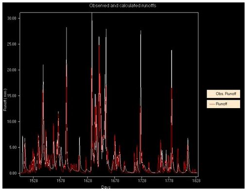
Figure 2. Observed and Modelled Daily Hydrograph (Coalburn – 1992-2003 excerpt)

Figure 3. Observed and Modelled Hydrograph (Coalburn 30 minute Flow excerpt)

Figure 4. Observed Vs. Modelled Monthly Volumes (Coalburn)

Figure 5. Observed Vs. Modelled Daily Volumes (Coalburn)
The above figures illustrate several issues that were present in calibrating MUSIC to sub-daily flow data. It can be seen that the daily and monthly flow scatter graphs in Figures 4 and 5 above show a reasonable fit, with Nash Sutcliffe Efficiencies (NSE) of 0.671 for daily and 0.931 for monthly flows using SimHyd. This again is well illustrated by the daily flow time series presented in Figure 2. When looking at the sub-daily flow however, as shown in Figure 3, it was obvious that the model response is correct (ie. runoff is being generated at the right level of magnitude for a particular rainfall occurrence), however the model is unable to represent base flow recession well.
This is due to the fact that the MUSIC hydrologic model is a daily model with disaggregation to the sub-daily time-step shown, where the runoff value for each time-step is calculated by dividing the daily flow by the portion of daily rainfall which fell in that time-step according to the process outlined earlier in this Appendix. As such, no routing of flows through the hydrologic model occurs at the sub-daily time-step and hence it will not be able to reproduce the characteristics of the sub-daily flow curve, though the response and magnitude of the peak flows is approximately representative of the observed data.
It is therefore suggested that the rainfall runoff model in MUSIC can reasonably predict the magnitude and response of peak flows within the UK context, however it will not represent the sub-daily flow characteristics well. These observations were shown to hold well for the Ravensbourne, Coalburn and Eastwood Brook catchments, however the Costa Beck catchment showed a very significant low bias in representing flows and no suitable calibration was able to be obtained. On further investigation of this, it was obvious that a significant baseflow was being indicated on the flow gauge, however again, MUSIC was able to represent the flow response reasonably well, albeit offset by the amount of baseflow indicated by the gauge. This is shown in the figure below:

Figure 6. Costa Beck Observed and Predicted Flow
When calculated, it was identified that the runoff measured in the gauge was approximately three times the rainfall volume, which indicated either the gauge is not recording the correct values, or there is a large groundwater intrusion into the stream. It was still obvious from the above that model is responding appropriately to rainfall by generating appropriate surface runoff pulses, however no further information could be derived for that catchment.
MUSIC Calibration Implications in Ungauged Catchments
During the calibration process, several issues became obvious in determining appropriate hydrologic parameters. In the urbanised catchments such as Ravensbourne and Eastwood Brook, the catchment imperviousness as determined using the process outlined previously yielded an appropriate level of catchment runoff that matched the gauged record well. In the rural catchments with low levels of built up areas, it was obvious that parts of the catchment were acting as impervious surfaces, indicating that there may be periods where soils were fully saturated (e.g. during prolonged winter rainfall) and therefore the pervious areas were generating higher amounts of surface runoff. This also showed that the soil stores were likely to be relatively shallow in these areas. As such, in order to yield a suitable flow equivalent to that seen in the gauged record, the percentage impervious factor in the source node was adjusted until suitable runoff volumes were obtained. This indicates that in order to obtain indicative flows from catchments with little or no impervious surfaces, the impervious percentage should be adjusted to match typical runoff coefficients for that type of catchment. The impervious percentage should therefore be considered to act more like a runoff coefficient factor than a direct relationship to catchment imperviousness.
What was also obvious during the calibration process on the rural catchments was that the field capacity had a significant influence on the runoff generated. From this, it was determined that the when field capacity was set at 1/3 of the soil storage capacity, the field capacity was less influential on runoff and the runoff coefficient/percentage imperviousness value once again was the dominant parameter in determining suitable runoff response.
Appropriate UK default parameters were derived by examining the results of the parameterisation and calibration tasks. The defaults are not intended to replace local parameterisation using the methods outlined above, but would allow initial parameters for UK MUSIC model runs to be based UK data rather than Australian data. It should be noted that users are strongly recommended to parameterise the model for their modelling location rather than rely on these default values.
References
- Packman, J. C., 1980., Report No. 63 - The effects of urbanisation on flood magnitude and frequency, Institute of Hydrology, Wallingford.
- http://www.ceh.ac.uk/data/nrfa/data/spatial.html?37033