About storage routing
Storage routing is based on mass conservation and the assumption of monotonic relationships between storage and discharge in a link.
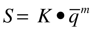
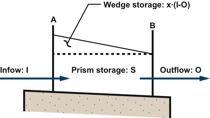
This is a simplification of the full momentum equation and assumes that diffusion and dynamic effects are negligible. The method uses index flow in flux, storage and mass balance equations. A weighting factor is used to adjust the bias between inflow and outflow rate, hence allowing for attenuation of flow. The storage routing equation is shown below and some of its terms are represented diagrammatically in Figure 1.
| Equation 1 |
|---|
where:
S is the storage in the reach,
k is the storage routing constant
m is the storage routing exponent, and
q~ is the index flow, which is given by
| Equation 2 |
|---|
where:
I is the inflow to the reach during the time-step,
O is outflow from the reach during the time-step and
x is the inflow bias or attenuation.
Figure 1. Prism and wedge storage
Dead storage
Dead storage refers to the capacity of a storage that is below the minimum operating level. At this water level, there is no outflow. The level of the reach with respect to dead storage at the beginning of the time-step affects its level in subsequent time-steps as follows:
- The reach is at or below dead storage and the fluxes during the time-step are insufficient to raise the level above the dead storage;
- The reach is above dead storage but fluxes during the time-step would lower the level in the reach below dead storage; or
- The reach is above dead storage and remains above dead storage during the time-step.
To determine if the reach is at or below the dead storage level, Source:
- Computes an initial storage estimate by using inflows to fill the reach up to but not exceeding the dead storage level;
- Computes a revised storage estimate based on any remaining inflows and fluxes, but ignoring outflows; or
- If the revised storage estimate is above dead storage, then outflows are computed. Otherwise, the initial storage estimate is used and outflows are set to zero.
Initial Estimation of Storage Constant (k)
An initial value of k can be determined by
- For linear routing (ie m=1) k is equal to the wave travel time divided by the number of divisions. The wave travel time is how long the wave takes to move through the reach
- For non-linear routing, (m≠1) k can be calculated using the known wave travel time for the reach and the chosen value of m for a representative flow rate
| Equation 3 |
|---|
where:
Tw is the known travel time for the reach in seconds
n is the number of divisions
Qw is the flow rate at which you want the travel time to be Tw in m3/s.
Configuring storage routing
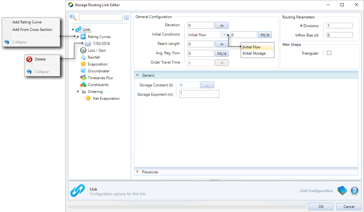
Figure 2 shows the feature editor for storage link routing and Table 1 outlines the parameters required.
Figure 2. Storage routing link
Table 1. Parameters for link storage routing
| Parameter | Description | Units | Range | Default |
|---|---|---|---|---|
| General configuration | ||||
| Avg. Reg. Flow | Average regulated flow is used to calculate travel time for orders in the ordering phase. It is not used in the flow distribution phase. | megalitres per day | real ≥ 0 | 0 ML/d |
| Elevation | Note that while it is usual to use zero storage as the reference point for the elevation of a link or node, there is no convention for a link as to whether that should be at the start or end of the reach, or some point in between. Source has no mechanism for indicating the fall across a reach. | |||
| Initial conditions | If necessary, one of these parameters may be used to seed a reach with either an initial flow or storage (see below) so that reach behaviour is fully defined from the first model time-step. | |||
| Initial flow | megalitres per day | real ≥ 0 | 0 ML/d | |
| Initial storage | The amount of water deemed to be in the link on the first time-step. For example, if there is a lag of two days, and there is 10ML in the link at the start of the run, then 5ML is deemed to be flowing out each day (total initial storage divided by lag). | megalitres | real ≥ 0 | 0 ML |
| Reach length | Source simulates evaporation and rainfall using the user defined reach length and a reach width (based on simulated flow and a user defined rating curve) to calculate surface area. | metres | real ≥ 0 | 0 m |
| Routing parameters | ||||
# Divisions | Number of reach divisions. Conceptually, this parameter describes the number of times that a reach is replicated. The effective length of a reach is determined from its behaviour, which is controlled by the combination of the storage exponent m, the inflow bias x and the storage constant K. Specifying multiple reach divisions implies applying the same set of behavioural parameters multiple times. In other words, if the effective length of a single-division reach is 500 metres (as derived from its behavioural parameters), changing the # Divisions parameter to 2 implies a combined effective length of 1000 metres. If you want to sub-divide a 500 metre reach into two 250 metre sections, you must also change the behavioural parameters to achieve this. | whole units | integer ≥ 1 | 1 |
| Inflow bias (attenuation factor, x) | The weighting factor x is used to adjust the bias between inflow and outflow rate and allows for flow attenuation. The weighting factor is usually in the range 0 ≤ x ≤ 0.5 (Davis and Sorensen, 1969). A recommended starting value is 0.2. | dimensionless | real 0 ≤ x ≤ 1 | 0 |
| Generic | ||||
| Storage constant (k) | When using linear routing (m = 1), the units of the storage constant k are in seconds and the wave travel time is equal to k times the number of divisions. When using non-linear routing (m ≠ 1), a starting value could be calculated using Equation XX in the scientific reference guide. | k units | real ≥ 0 | 0 |
| Storage exponent (m) | If m=1, linear (Muskingum) routing is implied, otherwise non-linear routing is implied. m=0.74 is a good starting value for a natural channel. | time-steps | real 0 < m ≤ 1 | 0 time-steps |
Piecewise storage function
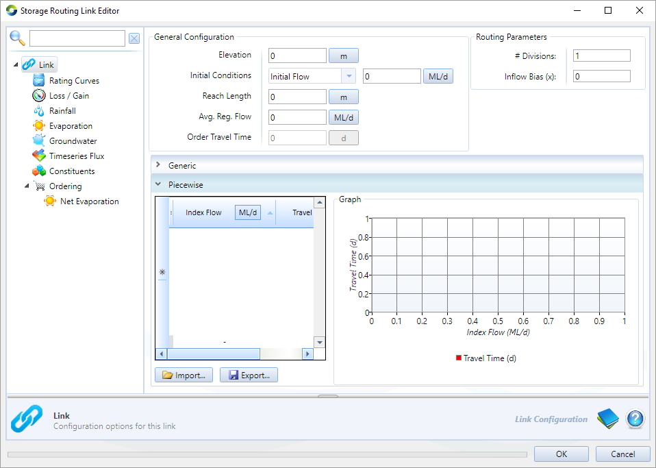
Flow travel time can also be set using a piecewise linear function. This describes a series of relationships between reach index flow rate versus travel time. The data points can be entered manually or imported from a .CSV file, the format of which is shown in Table 2. See the SRG for details: Link storage routing - SRG.
To get hydraulically valid results, the maximum travel time can not be more than the timestep divided by the inflow bias ( x ) per division. For example in a daily model, if you have three divisions and x = 1, the maximum travel time can be no more than 3 days. If x = 0.5 the maximum travel time could not be any more than 6 days
Figure 3. Storage routing link, Piecewise
Table 2. Storage routing link, Travel time (data file format)
| Row | Column (comma-separated) | |
|---|---|---|
| 1 | 2 | |
| 1 | Index flow | Travel time |
| 2 … n | flow | day |
Link rating curve
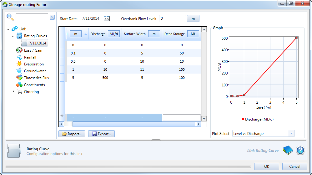
Rating curves (Figure 4) are used to describe the physical characteristics of the reach and convert a flow into a level, ie. they produce an output of level. They can be specified in one of two ways:
- Using the Cross Section Editor to specify a physical cross section, and then generating the rating curve; or
- Directly entering the rating curve - the piecewise linear editor allows you to define relationships with respect to water level, discharge rate, reach width and dead storage. You can define multiple rating curves for a reach, each scheduled to commence on a particular date.
To define a new rating curve directly:
- Right click Rating Curve and choose Add Rating Curve;
- Today’s date will automatically be entered for Start Date. To change this, click the calendar on the right side (see Working with date-pickers);
- Enter the water level, discharge rate, reach width and dead storage; and
- Enter an appropriate value for Overbank Flow Level.Error rendering macro 'jira' : Unable to locate Jira server for this macro. It may be due to Application Link configuration.
Figure 4. Storage routing link, Rating curve
You can also use the Import button to import a rating curve from a .CSV file the format of which is shown in Table 3.
Table 3. Storage routing link, Rating curve (data file format)
| Row | Column (comma-separated) | |||
|---|---|---|---|---|
| 1 | 2 | 3 | 4 | |
| 1 | Level | Discharge (ML/d) | Surface width (m) | Dead storage (ML) |
| 2 … n | level | rate | width | storage |
where:
level is the storage height in the reach in metres above a datum
rate is the outflow from the reach in the corresponding level
width is the surface width of the reach at the corresponding level
storage is the dead storage in the reach at the corresponding level
There should be at least one row describing the maximum depth at which there is zero flow, and which quantifies the maximum amount of dead storage in the reach. Thereafter, the dead storage volume should remain constant. Table 4 shows an example of this. A depth of 0.5 metres defines the maximum amount of dead storage (100 megalitres), after which the dead storage remains constant. Note that if discharge is 0, then dead storage must be increasing, or it must be equal to the previous value of dead storage.
Table 4. Storage routing link, Rating curve (example)
| Level (m) | Discharge (ML/d) | Surface width (m) | Dead storage (ML) |
|---|---|---|---|
| 0 | 0 | 0 | 0 |
| 0.1 | 0 | 5 | 50 |
| 0.5 | 0 | 10 | 100 |
| 1 | 10 | 11 | 100 |
| 5 | 500 | 15 | 100 |
To edit an exising rating curve, select the curve from the list of available curves under Rating Curve. Edit the data and click OK to close the editor. To delete a rating curve, right click the curve from the list and choose Delete.
You can also export rating curves to .CSV files by clicking the Export button.
Link losses and gains
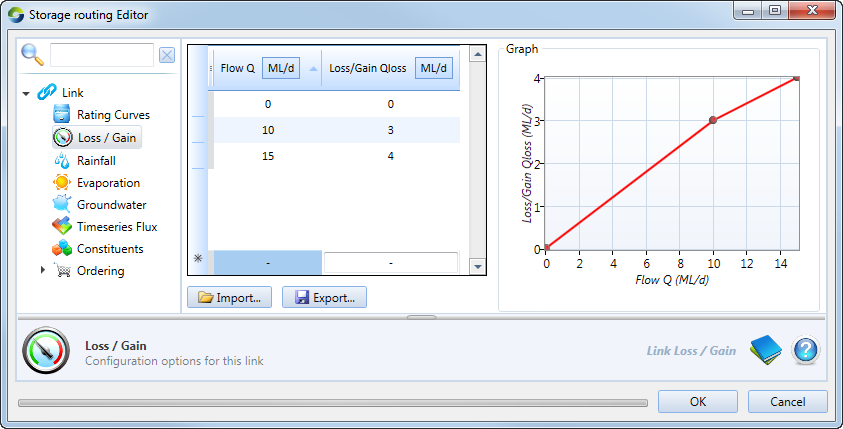
Choose Loss/Gain to specify flux as a function of flow using a piecewise linear editor. By convention, losses are described using positive numbers whereas gains are specified using negative numbers. In other words, a gain is a negative loss.
Figure 5. Storage routing, Loss/Gain
Link Evaporation
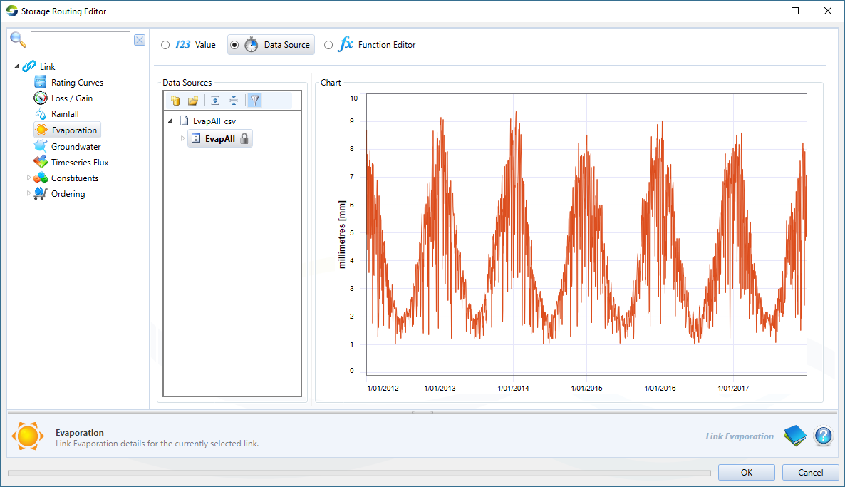
Choose Evaporation to specify the rate of evaporation per unit of surface area (Figure 6). Typically, this is done using a time series (loaded using Data Sources), the format of which is shown in Table 5. You can also specify the rate of evaporation as a single value or as a function.
Figure 6. Storage routing, Evaporation
Table 5. Storage routing link, Evaporation (data file format)
| Row | Column (comma-separated) | |
|---|---|---|
| 1 | 2 | |
| 1..n | time | value |
where:
time is the time of obersvation in "dd/mm/yyyy hh:mm:ss" format
value is the evaporation rate in millimetres per time-step
Groundwater
Choose Groundwater to configure groundwater models on the storage routing link. Refer to Groundwater.
Constituents
Choose Constituents to configure constituents on the storage routing link. Refer to Constituents - Links.
Timeseries Flux
Choose Timeseries Flux to configure flux as a value, data source or function.
The Timeseries flux can be a loss or a gain, adjustments to orders can be enabled under ordering.
Ordering at links
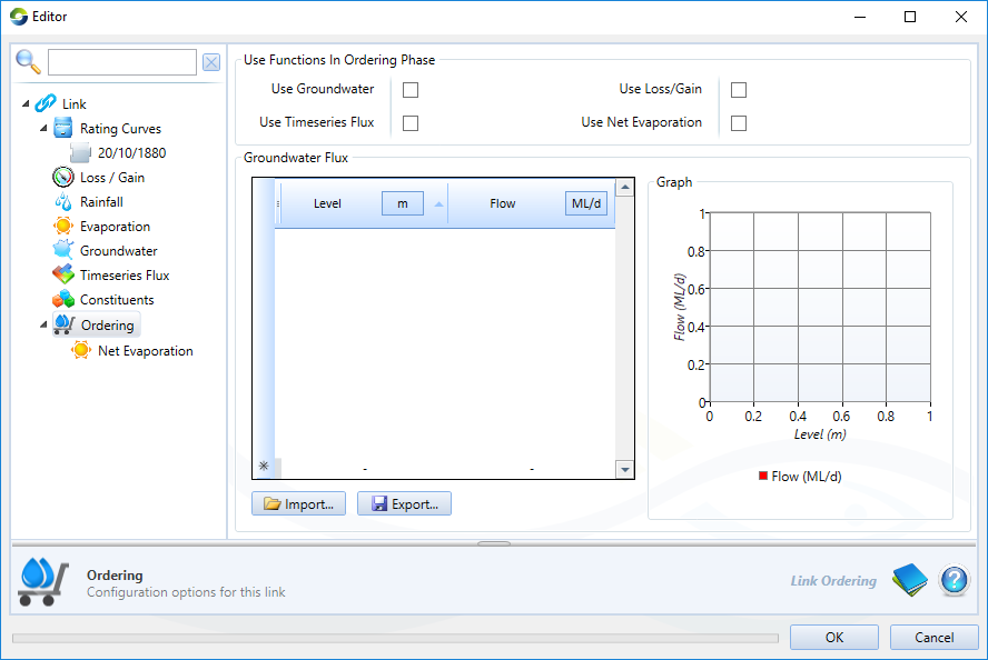
Choose Ordering and configure the parameters as shown in Figure 7.
Figure 7. Link (Ordering)
Ownership at links
Ownership must be enabled at the scenario-level (using Edit » Ownership) prior to configuring ownership at storage routing links. Refer to Ownership for details.
References
Davis, C.V., and K.E. Sorensen (1969) Handbook of Applied Hydraulics, 3rd Edition, C.V. Davis and K.E. Sorensen (eds). McGraw-Hill.
