Appendix G: Selecting Appropriate k and C* Values
Introduction
The selection of appropriate k and C* values for music is an important consideration in simulating any proposed treatment measure. This appendix gives guidance on selection of k and C* values, based on:
- A theoretical framework, outlined in the section on Guiding Principles;
- Evidence from recent Australian calibration studies, outlined in Evidence from Recent Calibration Studies.
- Recommended values derived from a synthesis of a and b (Selecting Appropriate k and C* Values).
At this stage the selection of default values for k and C* for music is therefore based on a combination of hypothetical (qualitative) and limited quantitative information, owing to the absence of any extensive data base for the range of stormwater treatment measures considered. Nevertheless, default values are required, and should address both the relative effectiveness of the various treatment nodes, and the relative behaviour of the different water quality parameters at a single node. This Appendix describes how the default values of k and C* were derived.
In this Version 3 of music, we have, where data are available, provided more guidance on appropriate ranges of k and C* values. Notwithstanding this, users are strongly encouraged to calibrate music to observed (monitored) data wherever possible, and to search for relevant studies which may provide guidance.
Guiding Principles
The theoretical framework provided in the following six sections provides an "upper limit" of expected treatment performance. There are a number of reasons why lower treatment may be observed (e.g. variations in PSD, breakdown of Stokes’ Law for small particles, etc), and the user should refer to Evidence from Recent Calibration Studies and Selecting Appropriate k and C* Values, before selecting final k and C* values.
The notional values of k and C* for the various treatment measures modeled in the USTM using the 1st order kinetic model should reflect the following broad principles:
- the relative values of k for each of the facilities in the treatment train should reflect the settling velocities of the targeted sediment size; C* for each of these facilities should reflect the particle size range which the respective treatment measures are not normally designed to remove.
- the relative value of k for TP and TN with respect to TSS for each treatment facility should reflect the speciation of these water quality constituents by the particle size range of the suspended solids.
- where users are unsure, a conservative approach should used (ie. selection of lower k values, and higher C* values).
A possible approach to determining appropriate k and C* values could be based on first assuming a representative particle size distribution of suspended solids (sediment) in urban stormwater and an assumed pollutant speciation distribution within this range (see Particle Size Distribution).
It should be noted that the k-C* modelling approach adopted in the USTM is currently strictly applicable only during event operation. The parameter k lumps together the influence of a number of predominantly physical factors on the removal of stormwater pollutants. While the assumption of a predominance of physical removal processes during storm event operation is reasonable for particulate (inorganic) contaminants, other factors associated with chemical and biological processes can also be significant. These are currently not accounted for in the determination of k.
The background concentration C* is assumed to be a constant at present although intuitively we would expect C* to be influenced by hydraulic loading, flow velocity and other factors affecting the re-mobilisation and maintenance of suspended solids in stormwater. However, C* can be expected to also vary during the inter-event period as chemical and biological processes alter the ambient concentrations of contaminants in waterbodies receiving stormwater. These processes are not modelled in the current version of USTM, but are subject to-going research and development.
Particle Size Distribution and Sediment Settling Velocities
Both Melbourne and Brisbane catchments are characterised by fine particle size distributions of suspended solids. Figure 1 shows a typical distribution derived from field sampling of road runoff in an established fully developed catchment in Melbourne, which we have assumed to be representative of Melbourne and Brisbane catchments. The settling velocities computed using Stokes Law and Rubey’s Equation, are shown in Figure 2. A particle density factor ranging from 2.6 at 500 µm to 1.1 at 2 µm (Lawrence & Breen, 1998) has been incorporated into Figure 2. Even so, it should be noted that actual settling velocities in the field are often significantly lower than the theoretical values shown. This is particularly the case with fine particles, owing to the influence of water turbulence caused by wind and aquatic fauna.
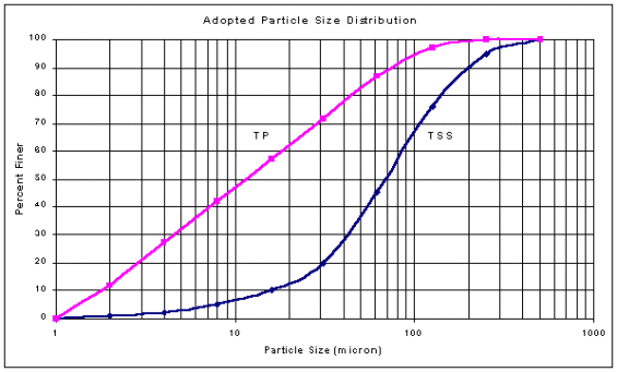
Figure 1. Possible PSD for Melbourne and Brisbane catchments (adapted from Lloyd et al, 1998).
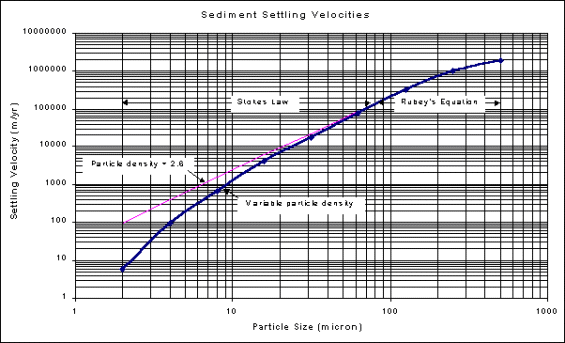
Figure 2. Theoretical settling velocities for sediments.
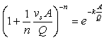
Fair and Geyer (1954) provided the following expression for computing the removal efficiency of suspended sediments in wastewater sedimentation basin design:
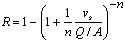 (1)
(1)
where
R fraction of initial solids removed
vs settling velocity of particles
Q/A rate of applied flow divided by the surface area of the basin or wetland
n turbulence and short-circuiting parameter (between 0 and 1)
The above expression attempts to account for the effects of water turbulence and non-uniform velocity distribution in the treatment facility by the turbulence and short-circuiting parameter n. The parameter n is a similar type of measure to the hydraulic efficiency of the treatment facility (Persson et al., 1999), related to the number of CSTRs:
 (2)
(2)
Thus a low short-circuiting factor n is associated with a low number of CSTRs and high turbulence, and high n is associated with near plug-flow conditions.
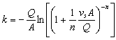
The equation of Fair and Geyer has, as an independent variable, the hydraulic loading of the system (i.e. Q/A) and we can adopt the Wong and Breen chart (Figure 3) to provide some guidance on the operating hydraulic loading range of the various treatment measures considered.
Rearranging the expression for the k-C* model gives:-
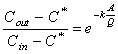 (3)
(3)
For the theoretical assumption that under ideal sedimentation conditions, C* should approach zero, the following expression can be derived by combining the two equations listed previously:
 (4)
(4)
However, it is unlikely that C* in the field will be zero owing to physical (eg. wind induced turbulence) and chemical/biological factors maintaining a "irreducible" concentration in most treatment measures.
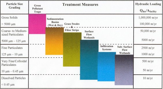
Figure 3 Operating hydraulic loading and target particle size of stormwater treatment measures (Wong, 2000).
Total Suspended Solids
Sedimentation basins are essentially ponds designed to remove larger particulates. According to Figure 3, the target sediment size is 125 µm or larger, with the system having some capability of removing finer particle sizes under lower hydraulic loading conditions. The theoretical settling velocity of a 125 µm sized sediment is of the order of 300,000 m/yr. The operating hydraulic loading range for sedimentation basins is between 5,000 m/yr and 50,000 m/yr.
The expected removal efficiency of suspended solids with a PSD as shown in Figure 1 can be computed using Equation (1) by sub-dividing the PSD into a number of various bands along similar groups as that illustrated in Figure 3. The expected removal of TSS for a typical hydraulic loading of 30,000 m/yr is approximately 31%, with more than half the particles larger than 125 µm removed, but only 20% of 30 mm particles removed. This is a reasonable outcome from the sedimentation basin, and gives a k value of 11,000 m/yr for C* equal to zero (Equation 3).
An estimate of C* can be obtained from the particle size at which only 20% removal is achieved. Under the specified conditions, this corresponds to a particle size of 30 µm, or 19% of the sediment concentration (from Figure 1), and leads to a k value of 15,000 m/yr. For an event mean concentration (EMC) of 160 mg/L (rounded from Duncan, 1999), C* becomes 30 mg/L.
Hence for TSS in a sedimentation basin we have k = 15,000 m/yr, and C* = 30 mg/L.
Constructed wetlands would normally follow sedimentation basins in a treatment train. These systems are subjected to inflow of suspended solids of finer PSD owing to the pre-treatment provided by the sedimentation pond and the typical range of hydraulic loading is between 50 and 5000 m/yr. The expected removal of TSS in a wetland with a typical hydraulic loading of 2,500 m/yr downstream of the sedimentation basin described above is approximately 81%, giving 87% removal by sedimentation basin and wetland together. Without the sedimentation basin, the wetland still achieves about 86% removal, but has significantly faster accumulation of sediment. Almost all particles larger than 62 µm are removed but only 20% of the 6 µm particles are removed. As above, the 20% removal threshold, 6 µm in this case, could be adopted as an estimate of C*. From Figure 1, particles finer than 6 µm constitute about 4% of the suspended solids in urban stormwater. An EMC of 160 mg/L TSS thus gives a C* value of 6 mg/L. The corresponding value of k is about 5000 m/yr.
Hence for TSS in a wetland we have k = 5,000 m/yr, and C* = 6 mg/L.
Ponds, Infiltration Systems and Rainwater Tanks are all assumed to be subject to some form of pre-treatment to remove coarse sediments. Owing to the significantly lower TSS concentration and the higher proportion of finer fractions entering such ponds, further water quality improvement is limited. For a pond with hydraulic loading of 500 m/yr, downstream of the sedimentation basin and wetland described above, Fair & Geyer’s sedimentation equation indicates a combined removal by all three facilities of 93%, and a C* (defined by 20% removal => 5 mm => 3%) of 5 mg/L for the pond. But we know from experience that resuspension by turbulence in open water becomes important at these small particle sizes. It seems preferable, therefore, to abandon the pure sedimentation mechanism at this point, and instead adopt a rule of thumb that C* in a pond is about twice that of a comparable wetland, or about 12 mg/L. The corresponding value of k is 1000 m/yr.
Hence for TSS in a pond we have a theoretical k = 1,000 m/yr, and C* = 12 mg/L
Swales are located nearer to the pollutant source and are used in the early stages of the treatment train. The modelling of the performance of swales will be similar to that for a wetland (with 10 CSTRs) but probably subjected to a more variable hydraulic loading of between 500 m/yr and 30,000 m/yr. Intuitively, owing to a higher aspect ratio, swales will experience higher velocities even when subjected to relatively low hydraulic loading. The Fair and Geyer equation will not be able to simulate this and it will be necessary to qualitatively account for this process when selecting the appropriate value of C* for swales.
Although swales are somewhat similar to wetlands in their flow regime, they are more similar to sedimentation basins in their position in the treatment train, and hence in their likely particle size distribution. For the time being, it seems appropriate to adopt for swales the same k and C* parameters as for sedimentation basins, but with higher N (number of CSTRs) to reflect the more plug-like flow behaviour.
Hence for TSS in a swale we have k = 15,000 m/yr, and C* = 30 mg/L.
Theoretical values of k and C* for TSS are summarised in the table of recommended values presented in Selecting Appropriate k and C* Values.
Total Phosphorus
The removal efficiency of phosphorus during storm events can be assumed to be primarily associated with the removal of TSS. Urban water quality data have indicated that a high proportion of TP in urban stormwater is in particulate form. For this study, phosphorus is assumed to be distributed over the particle size range in proportion to the surface area of particles of each size range. Combined with the adopted TSS particle size distribution in Figure 1, and smoothed slightly, this produces the TP curve also shown on Figure 1. There has been little emphasis placed on the distribution of particles less than about 2 microns, because under the sedimentation approach adopted, they are never likely to settle anyway.
The k and C* values for total phosphorus have been calculated using the same approach as for TSS, using the TP distribution curve from Figure F-1, and the Australian EMC of 0.26 mg/L (Mudgway et al., 1997). The results are summarised in Appendix G: Selecting Appropriate k and C* Values. The values of k are consistent with the expectation that they should be lower than corresponding values for TSS.
Theoretical k and C* values for TP are summarised in the table of recommended values presented in Appendix G: Selecting Appropriate k and C* Values.
Total Nitrogen
The selection of appropriate k and C* values for modelling the removal of Total Nitrogen can not easily follow the procedure applied for TSS and TP. The composition of particulate and soluble forms of N in stormwater is highly varied. There is significantly smaller particulate fraction of TN compared with TP, and even that fraction is associated with organic particles which have significantly lower specific gravities than sediment. Calibrated k values for TN in wastewater systems indicate significantly lower values (as much as two orders of magnitude) compared with TP and TSS.
The default k and C* values for TN are thus based on very limited data. There is an expectation that the k values are likely to be an order of magnitude lower than corresponding values for TP, and that the ratios of C* to inflow EMC are likely to be higher for TN than for TP.
Theoretical k and C* values for TN are summarised in the table of recommended values presented in Appendix G: Selecting Appropriate k and C* Values.
Developing Catchments
The theoretical k and C* values have some important inherent assumptions related to the particle size distribution of the suspended sediment in stormwater and the speciation of particulate phosphorus to the particle size fractions (as depicted in Figure 1). It is possible that the particle size distribution will be different for catchments of different geology, particularly if the catchment is undergoing urbanisation with scattered construction activities throughout the catchment. A likely typical PSD for developing catchments is shown in Figure 4. The resulting theoretical values of k and C* are listed in Table 1.
Figure 4. Possible PSD for developing catchments in Melbourne and Brisbane.
Table 1. Summary of Estimated k and C* values for Developing Catchments.
Treatment Measure | TSS | TP | TN | |||
|---|---|---|---|---|---|---|
k (m/yr) | C* (mg/L) | k (m/yr) | C* (mg/L) | k (m/yr) | C* (mg/L) | |
Sedimentation Basins | 15,000 | 95 | 12,000 | 0.22 | 1,000 | 1.7 |
Ponds | 300 | 40 | 200 | 0.20 | 50 | 1.3 |
Swales | 15,000 | 95 | 12,000 | 0.22 | 1,000 | 1.7 |
Wetlands | 3,200 | 32 | 2,100 | 0.10 | 500 | 1.3 |
It can be seen that a finer PSD leads to less effective treatment – lower k, higher C*, or both. Hence when a finer PSD is believed to be present, values of k and C* interpolated between those in Tables 3 and 4 may be more appropriate. When selecting appropriate k and C* values (using the recommendations in Appendix G: Selecting Appropriate k and C* Values), consideration should be given to the adjusted theoretical values in Table 1.
Evidence from Recent Calibration Studies
The theoretical framework for selecting k and C* values presented in the previous sections has been tested through a number of recent studies where observed inflow and outflow data from stormwater treatment measures were analysed.
This section outlines four Australian studies undertaken to calibrate music to observed data:
- Vegetated swale in Brisbane (Pinjarra Hills Estate)
- Stormwater pond / lake in Melbourne (Blackburn Lake)
- Large constructed wetland in Melbourne (Hampton Park Wetland)
Brisbane Swale - Pinjarra Hills Estate
Introduction
Brisbane City Council, with assistance from the CRC for Catchment Hydrology, conducted a series of controlled field experiments, to test the removal of TSS, TP and TN from a short swale in a residential estate. Due to a number of limitations of the experiment, only the results from TSS have been able to be reliably used for the calibration of music. This has been done with the aid of a deterministic sediment transport model called TRAVA.
Study Site
The experimental site was located in a residential estate at Pinjarra Hills in Brisbane, along a 65m long swale (Figure 5), with a longitudinal slope of 1.6%, batter slopes of approximately 1:13, and a catchment area of 1.03ha. The swale had a top width of 4m, and was approximately triangular in cross-section. It contained a mix of winter rye and couch grass, with average aerial cover of 67%. Sampling points were located every 16.25m along the swale (Figure 5).
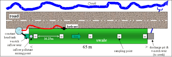
Figure 5. Experimental setup and sample locations.
Methods
(i) Field Experiments
A constant-head tank, discharging through a v-notch weir, provided steady flows ranging from 2L/s up to 15L/s (Table 2). The swale flow discharged to a pit, where a second v-notch weir was installed, to ensure steady-flow conditions were maintained, and calculate flow losses. Inflows were dosed with a synthetic pollutant mix over 5 minutes (plug inflow), matched to recently-observed Brisbane stormwater characteristics (in terms of concentration). However, the particle size distributions (PSDs) used were substantially less than ‘typical’ expected PSDs (refer to Note 1 of Table 1). Water samples were taken at the inlet, outlet and three points along the swale, for a period of fifty minutes. Samples were analysed for TSS, TP and TN, in a quality-accredited laboratory.
Two sets of field tests were carried out, in 2000/2001 and 2001/2002. The experimental conditions for the reliable experiments are presented in Table 1 (Brisbane City Council, 2005). The concentrations of pollutants in the inflow as well as sediment characteristics were within the range measured in Brisbane.
Some factors limited use of the data for calibrating music:
- The Particle Size Distributions (PSDs) used in the experiment were lower than typically expected in urban areas, because the analysis method used by BCC to report PSDs sieved out all particles larger than 90 µm prior to the analysis. The swale experiments then used synthetic sediment matched to this cropped PSD. Compared with Figure 1 in this Appendix, the PSDs used in the experiment (see Table 2) are towards the fine end; thus a lower k and higher C* than the ‘hypothetical values’ described in Particle Size Distribution et al. would be expected.
- Use of synthetic pollutants introduced potential artefacts which may not reflect observed behaviour of ‘natural’ stormwater.
- Dosing with tap water may introduce artefacts (e.g potentially lower C* than would be observed in reality)
- Irregular mixing in the inflows produced anomalies in the observed concentrations in the upstream part of the swale.
- The experiment’s short-dosing period was less than the minimum time-step in music.
Application of a deterministic modelling approach for TSS, using the model TRAVA (Deletic, 2001, Deletic 2005; Deletic & Fletcher, in press), was used to overcome several of these limitations. Given these anomalies, the results presented here replace previously reported results (Fletcher, 2002; Fletcher et al., 2001, Fletcher, et al., 2002). Interpretation of the results must also take into account the particle size distributions.
Table 2: Characteristics of reliable experiments carried out in Brisbane (BCC, 2005).
Run No | Swale Height & Density | Q (L/s) | PSD | Pollutant Inflow Conc. |
|---|---|---|---|---|
2000/2001 Experiments | ||||
Run 6 | Winter rye and Couch - mown 1 week prior to sampling | 2 | FINE* particle size - Silica 400G d10=2 μm d50=9.3 μm d90=23 μm | TSS = 150 mg/L, TN = 2.6mg/L, and TP = 0.3mg/L |
Run 7 | 5 | |||
Run 8 | 8 | |||
Run 9 | 12 | |||
Run 10 | 15 | |||
2001/2002 Experiments | ||||
Run 11 | Predominantly Couch, with a height of 100-150 mm | 5 | FINE* particle size - Silica 400G d10=2 μm d50=9.3 μm d90=23 μm | TSS: 150 mg/L N: 2 mg/L P: 0.3 mg/L |
Run 12 | 10 | |||
Run 13 | 15 | |||
Run 14 | 10 | TSS: 80 mg/L N: 0.6 mg/L P: 0.1 mg/L | ||
Run 15 | 10 | TSS: 250 mg/L N: 3.4 mg/L P: 0.6 mg/L | ||
Run 17 | 5 | MEDIUM* - Silica 60G d50=approx. 43 μm |
| |
Run 19 | 10 | |||
Run 21 | 15 | |||
* NOTE 1: In the BCC reporting of these experiments (Brisbane City Council, 2005), the “Fine” Sediment was referred to as “standard” and the “Medium” was referred to as “Coarse”. These have been re-named to better describe their relationship to typical observed PSDs (refer to Figure 1).
(ii) Data Analysis
TSS analysis:
- Only the data collected at the swale outflow were used.
- TRAVA was used to prepare the data for calibration of music:
- TRAVA was verified for the Brisbane swale ( runs listed in Table F-2)
- TRAVA was used to model steady-state outflows of sediment at the swale outflow as if the known sediment concentration had been added to the inflow over prolonged period, with all other conditions kept as in runs R11-15, R17, R19 and R21 (the aim was to compare the measured peaks and the modelled steady state outflow that would have been achieved if the sediment could have been added into the inflow over 1 hours; not just 5 minutes)
- TRAVA was used to model steady-state outflows of sediment for runs R11-15, R17, R19 and R21 but constant sediment inflows into a 200m long swale (with other characteristics same as the Brisbane swale), to assess the impact on C*.
- The TRAVA results were used to calibrate music. The best fit for k-C* was determined for two extremes of CSTRs = 1 & 10 (the latter recommended for swales). The sum of squares of the differences between TRAVA and music results was used as an objective function in the calibration process.
TP and TN analysis:
For nutrients, the k values are considered to be unreliable, but C* values were able to be derived, using a best-fit (sum of squares) to the observed data.
Results
TRAVA verification
TRAVA was used without calibration. For 2000/2001 experiments the modelled TSS concentrations in outflow were within ±17 % of measured, while the predicted mass of total TSS outflow was within ±11 % of measured. For 2001/2002 experiments the modelled load was within ±21 % of measured. Taking into account accuracy of TSS measurements (± 30%) it was concluded that TRAVA reliably predicts concentrations of TSS in Brisbane swale experiments.
music calibration
Table 3 presents the calibrated k and C* against the TRAVA simulated TSS concentrations along 200 m long swale (other characteristics as the Brisbane swale), and for steady state inflow of TSS (with the same characteristics as in the Brisbane swale experiments).
Table 3: Calibrated k-C* against TRAVA results
Run | q [l/s] | C-inflow | CSTRs=1 | CSTRs=10 | ||
|---|---|---|---|---|---|---|
[mg/l] | K [m/year] | C* [mg/l] | K [m/year] | C* [mg/l] | ||
FINE sediment | ||||||
R11 | 5 | 150 | 3950 | 26 | 2200 | 25 |
R12 | 10 | 150 | 5790 | 32 | 2500 | 25 |
R13 | 15 | 150 | 7000 | 30 | 3000 | 25 |
R14 | 10 | 80 | 5789 | 17 | 2500 | 13 |
R15 | 10 | 250 | 5787 | 53 | 2500 | 43 |
Average |
|
| 5663 | 31 | 2540 | 26 |
MEDIUM sediment | ||||||
R17 | 5 | 150 | 7073 | 5 | 4000 | 3 |
R19 | 10 | 150 | 10657 | 9 | 4000 | 3 |
R21 | 15 | 150 | 13056 | 11 | 7000 | 3 |
R22 | 10 | 80 | 10647 | 5 | 4500 | 3 |
R23 | 10 | 250 | 10635 | 15 | 3800 | 3 |
Average |
|
| 10414 | 9 | 4660 | 3 |
It is clear that k and C* depend on particle size (as discussed in Guiding Principles) and k also depends on flow rate (increasing with an increase of inflow rate), while C* is sensitive to inflow concentration. Most importantly, as discussed in The Universal Stormwater Treatment Model (USTM), k and C* both depend on the number of CSTRs. Variations in the reported values for k and C* for CSTRs=10 (usually recommended for swales) are much smaller than for CSTRs=1. This reinforces that selection of the appropriate value for Ncstr is a critical prerequisite for calibrating k and C*.
For TP and TN, C* values were derived:
- TP: C* ranged from 0.08-0.11 (average = 0.10) mg/L
- TN: C* ranged from 1.1-1.2 (average = 1.1) mg/L
Conclusions – Implications for calibration of music
For all reasonably long swales CSTRs should be 10. For CSTRs=10, Table 4 summarises the k and C* values observed for the Brisbane swale. The extent to which the recorded variations in k and C* will affect the modelled performance of a proposed swale, should be assessed using sensitivity analysis.
Table 4: Range of observed TSS k-C* for CSTRs=10.
TSS characteristics in the inflow | Inflow TSS concentrations | |||
Low | Medium | High | ||
Particle size | Fine d50= approx. 10 μm | K= 2500 m/year C*=15 mg/l | K= 2500 m/year (2200-3000) C*=25 mg/l | K= 2500 m/year C*=45 mg/l |
Medium d50= approx. 45 μm | K= 4500 m/year C*=3 mg/l | K= 4500 m/year C*=3 mg/l | K= 3500 m/year C*=3 mg/l | |
Blackburn Lake, Melbourne
Study Site
Blackburn Lake is located on a tributary of Gardiners Creek, in an established urban area in the eastern suburbs of Melbourne. The lake was created in 1888 for agricultural water supply and recreational purposes. The outlet was modified in 1963 to assist with flood mitigation, and now comprises a circular glory hole spillway with a rectangular low flow orifice cut in the side.
The major land uses are residential (48%) and industrial/commercial (40%), with most of the remainder being open space surrounding the lake. Total catchment area is 296 hectares. Long term average annual rainfall in the catchment is 700 to 800 millimetres.
An extensive monitoring program was carried out in 1996 and 1997, recording inlet and outlet flows and water quality for a total of 56 events, together with low flow and in-lake monitoring (RossRakesh et al., 1999).
music Calibration
Blackburn Lake is an on-stream storage, with a spillway at the downstream outlet and no bypass facility. This layout is best fitted in music using a Pond treatment node. music was fitted visually, using the Observed Data function to import monitoring information, then adjusting parameters to optimise the fit between observed and modelled time series graphs.
There are three parameters to be fitted – the number of CSTRs (N), the background concentration of a given water quality measure (C*), and the corresponding exponential decay parameter (k). N is optimised first, by considering the timing and shape of outflow pollutographs. At this site, N = 2.
The background concentration C* is optimised next, followed by the decay parameter k. Some iteration may be needed to optimise both C* and k. The adopted values are shown in Table 5 below.
Hampton Park Wetland, Melbourne
Study Site
Hampton Park Wetland is a large stormwater treatment wetland on the southeastern fringe of Melbourne. Inlet ponds on two main inlet branches control flow into the wetland, and divert excess flows into diversion channels flanking the main wetland. The inlet branches below the diversion ponds have alternating zones of deep and shallow macrophytes. The main wetland below their confluence also includes zones of open water. Excluding the small inlet ponds, the wetland has a total surface area of 53,600 square metres, a permanent pool volume of 14,600 KL, and an extended detention volume of 35,300 KL.
The catchment area is rapidly urbanising rural land, with a total catchment area of 11.8 square kilometres. The area immediately surrounding the wetland is fully urbanised.
An intensive monitoring program commenced in July 2003, measuring water quality and flows at inlets and outlet, and quality at intermediate points along the wetland (Fletcher et al., 2004).
music Calibration
music was fitted visually, using the Observed Data function to import monitoring information, then adjusting parameters to optimise the fit between observed and modelled time series graphs. A storage with upstream diversion of high flows is best fitted in music using the wetland node.
The number of CSTRs (N) is fitted first. N = 5 was found to give satisfactory results. Background concentration C* and decay parameter k are fitted next, with iteration if necessary. The optimised values are shown in Table 5.
Selecting appropriate k and C* values
Recommended Ranges
The theoretical framework presented in Guiding Principles and the calibration results presented in Evidence from Recent Calibration Studies are summarised in Table 5. These have been used to derive recommended ranges for k and C*. The rationale for these recommendations is given below. The default values in music have been selected from these recommended ranges, based upon:
- Distributions of the populations of k and C* values (thus means are initially calculated from the log-domain (for k) or normal domain (C*).
- Consideration of the ‘relativity’ between treatments, observed from field and laboratory studies.
Table 5: Summary of theoretical, observed and recommended k and C* values.
Treatment Node
| TSS | TP | TN | |||
k | C* | k | C* | k | C* | |
Wetland |
|
|
|
|
|
|
Theoretical | 5,000 | 6 | 2,800 | 0.09 | 500 | 1.3 |
Calibration (HP) | 500 | 5 | 300 - 500 | 0.03 | 50 - 100 | 0.9 |
Recommended | 500 - 5,000 | 5 - 6 | 300 - 2,800 | 0.03 - 0.09 | 50 - 500 | 0.7 - 1.3 |
Pond |
|
|
|
|
|
|
Theoretical | 1,000 | 12 | 500 | 0.13 | 50 | 1.3 |
Calibration (BL) | 200 - 300 | 15 | 150 - 300 | 0.05 | 30 - 50 | 0.7 |
Recommended | 200 - 1,000 | 12 - 15 | 150 - 500 | 0.05 - 0.13 | 30 - 50 | 0.7 - 1.3 |
Infiltration System |
|
|
|
|
|
|
Theoretical | 1,000 | 12 | 500 | 0.13 | 50 | 1.3 |
Recommended | 200 - 1,000 | 12 - 15 | 150 - 500 | 0.05 - 0.13 | 30 - 50 | 0.7 - 1.3 |
Rainwater Tank |
|
|
|
|
|
|
Theoretical | 1,000 | 12 | 500 | 0.18 | 50 | 1.7 |
Recommended | 200 - 1,000 | 12 - 15 | 150 - 500 | 0.08 - 0.18 | 30 - 50 | 1.1 - 1.7 |
Sedimentation Basin |
|
|
|
|
|
|
Theoretical | 15,000 | 30 | 12,000 | 0.18 | 1,000 | 1.7 |
Recommended | 4,000 - 15,000 | 10 - 30 | 3,000 - 12,000 | 0.08 - 0.18 | 250 - 1,000 | 1.1 - 1.7 |
Swale |
|
|
|
|
|
|
Theoretical | 15,000 | 30 | 12,000 | 0.18 | 1,000 | 1.7 |
Calibration (B) | 4,660 | 3 | - | - | - | - |
Recommended | 4,000 - 15,000 | 10 - 30 | 3,000 - 12,000 | 0.08 - 0.18 | 250 - 1,000 | 1.1 - 1.7 |
Bioretention System |
|
|
|
|
|
|
Theoretical | 15,000 | 30 | 12,000 | 0.18 | 1,000 | 1.7 |
Recommended | 4,000 - 15,000 | 10 - 30 | 3,000 - 12,000 | 0.08 - 0.18 | 250 - 1,000 | 1.1 - 1.7 |
Rationale for Selection
Wetland
For TSS, the range for k and C* represent the theoretical values (upper limit) and the observed calibration for Hampton Park Wetland (lower value).
For TP and TN, the range of k values represent the theoretical (upper) and observed calibration (lower) values. The same approach has been used for specification of the TP range of C*. The lower estimate of C* for TN has also been derived from the Hampton Park calibration, but adjusted to account for known high dry weather inflow concentrations of TN at that site (Fletcher et al., 2004).
Pond
The range of k and C* values for TSS, TP, and TN are derived from the theoretical values and observed calibration from Blackburn Lake.
Infiltration System
The infiltration system is assumed to be a downstream treatment measure, subject to pre-treatment to remove coarse sediment, and thus the k and C* ranges have been derived from those of a pond.
Rainwater Tank
The recommended ranges for rainwater tanks have been based on those for ponds, except that the C* for TP and TN are predicted to be higher, due to the reduced potential for biochemical removal processes. Therefore, the C* values for TP and TN in a tank have been derived from those of a sedimentation basin.
Sedimentation Basin
The recommended values for sedimentation basins have been chosen to reflect the hydraulic and sedimentation processes observed in these basins. Based on available evidence, these basins appear to have similar performance to that of swales, and so the recommended ranges of k and C* have been derived from those of swales.
Swale
Recommended range of k for TSS reflects the observed calibration results (where the number of CSTRs=10) and the theoretical value. The range reflects variations in (a) PSD (b) localised turbulence causing a breakdown in the underlying assumptions of Stokes’ Law and Rubey’s equations.
The observed TSS C* for the Brisbane swale calibration (3 mg/L) is considered to be an artefact of the (a) artificial sediment used, and (b) dosing with tap water. The recommended range has been selected to incorporate a reasonable lower estimate (10 mg/L).
For TP and TN, no calibrated k values were available. The range has thus been determined by (a) setting the theoretical value as the upper limit, and (b) setting the lower limit with the same upper:lower limit ratio as has been observed for TSS.
For TP and TN, specification of the lower C* value range came from the lowest observed values in the Brisbane swale experiment.
Bioretention System
The recommended ranges for bioretention systems have been derived from those of swales, assuming that the above-ground component of the bioretention system is similar to a swale.
Where the user wishes to build a bioretention system that is more like a basin (ie. like an infiltration basin) then appropriate k and C* values for the infiltration system should be selected.
Considerations for Selecting k and C* Values
When selecting appropriate k and C* values from the ranges given in Table 5, some important issues must be considered:
1. The k and C* values should be considered as “pairs”. That is, if a higher k value is chosen, then a correspondingly higher C* value should also be specified.
2. The k and C* values chosen for a given treatment system should reflect its location in the treatment train. For example, if an infiltration system is placed without any pre-treatment system upstream to remove coarse sediment and protect it from clogging, it would take k and C* values
similar to that of a sedimentation basin (reflecting that it now receives a greater proportion of coarse particles).
3. Users are strongly encouraged to use local data to calibrate the k and C* values of music.
4. Sensitivity analysis should be undertaken by the user, to determine the effect of changing the k and C* values on overall performance of a proposed treatment system.
References
Brisbane City Council (2005). SQIDs Monitoring Program Summary Report.
Deletic, A. (1999). Sediment Behaviour in Grass Filter Strips. Water Science & Technology, 39(9), pp. 129-136.
Deletic, A. B., & Fletcher, T. D. (in press). Performance of grass filters used for stormwater treatment - a field and modelling study. Journal of Hydrology.
Duncan, H.P. (1999), Urban Stormwater Quality: A Statistical Overview, Report 99/3, Cooperative Research Centre for Catchment Hydrology, February 1999.
Fair, G.M. & Geyer, J.C. (1954). Water Supply and Waste Disposal, John Wiley and Sons, New York, Vol. 2, 973pp.
Fletcher, T. D. (2002). Vegetated swales: simple, but are they effective? Paper presented at the Second Water Sensitive Urban Design Conference, Brisbane.
Fletcher, T. D., & Poelsma, P. (2003). Hampton Park Wetland monitoring report (No. Edition 1). Melbourne: Department of Civil Engineering, Monash University, Cooperative Research Centre for Catchment Hydrology and Melbourne Water Corporation.
Fletcher, T. D., Peljo, L., & Fielding, J. (2001, July 2001). Grass swales for stormwater pollution control. Catchword, 96, 8-11.
Fletcher, T. D., Peljo, L., Fielding, J., & Wong, T. H. F. (2002). The performance of vegetated swales. Paper presented at the 9th International Conference on Urban Drainage, Portland, Oregon.
Fletcher, T. D., Poelsma, P., Li, Y., & Deletic, A. B. (2004). Wet and dry weather performance of constructed stormwater wetlands. Paper presented at the International Conference on Water Sensitive Urban Design (proceedings on CD), Adelaide, Australia, 21-25 November, 2004, pp. 1-10.
Lawrence, I., and P. Breen. (1998). Design Guidelines: Stormwater Pollution Control Ponds and Wetlands. Cooperative Research Centre for Freshwater Ecology.
Li, Y., Deletic, A. B., & Fletcher, T. D. (2005). A novel approach in modelling performance of urban stormwater wetlands. Paper presented at the Hydrology and Water Resources Symposium, Canberra, Australia.
Lloyd, S.D., Wong, T.H.F., Liebig, T. and Becker, M. (1998), Sediment Characteristics in Stormwater Pollution Control Ponds, proceedings of HydraStorm’98, 3rd International Symposium on Stormwater Management, Adelaide, Australia, 27-30 September 1998, pp.209-214.
Mudgway, L. B., H. P. Duncan, T. A. McMahon, and F. H. S. Chiew. (1997). Best Practice Environmental Management Guidelines for Urban Stormwater. Report 97/7, Cooperative Research Centre for Catchment Hydrology, Melbourne.
Persson, J., Somes, N.L.G. & Wong, T.H.F. (1999). Hydraulic Efficiency of Constructed Wetlands and Ponds, Wat. Sci. Tech., Vol. 40, No. 3, pp. 291-300.
RossRakesh, S., Gippel, C., Chiew, F., & Breen, P. (1999). Blackburn Lake Discharge and Water Quality Monitoring Program: Data Summary and Interpretation. Report 99/13, Cooperative Research Centre for Catchment Hydrology, Melbourne.
Taylor, G. D., Fletcher, T. D., Wong, T. H. F., & Breen, P. F. (2005). Design of constructed stormwater wetlands: influences of nitrogen composition in urban runoff, and dissolved nitrogen treatment behaviour. Paper presented at the Hydrology and Water Resources Symposium, Canberra, Australia.
Wong, T.H.F. (2000), Improving Urban Stormwater Quality – From Theory to Implementation, Water – Journal of the Australian Water Association, Vol. 27 No.6, November/December, 2000, pp. 28-31.