Restriction Curves
About Restriction Curves
Once a system is in a certain state, an action occurs. For instance, if water supply levels drop below 50%, a set of water restrictions are imposed for a period of time. Restrictions or triggers can also be used to trigger events such as releases from a certain storage, desalination supply rates or environmental flows based on salinity levels. The aim of the trigger/restriction curves is to provide a time series that tracks what level of restriction the system is in. This time series can then be used to modify some other variable such as demand or inflow (desalination) as well as being a measure of the standard of service delivered. For detailed information, refer to the Source Scientific Reference Guide.
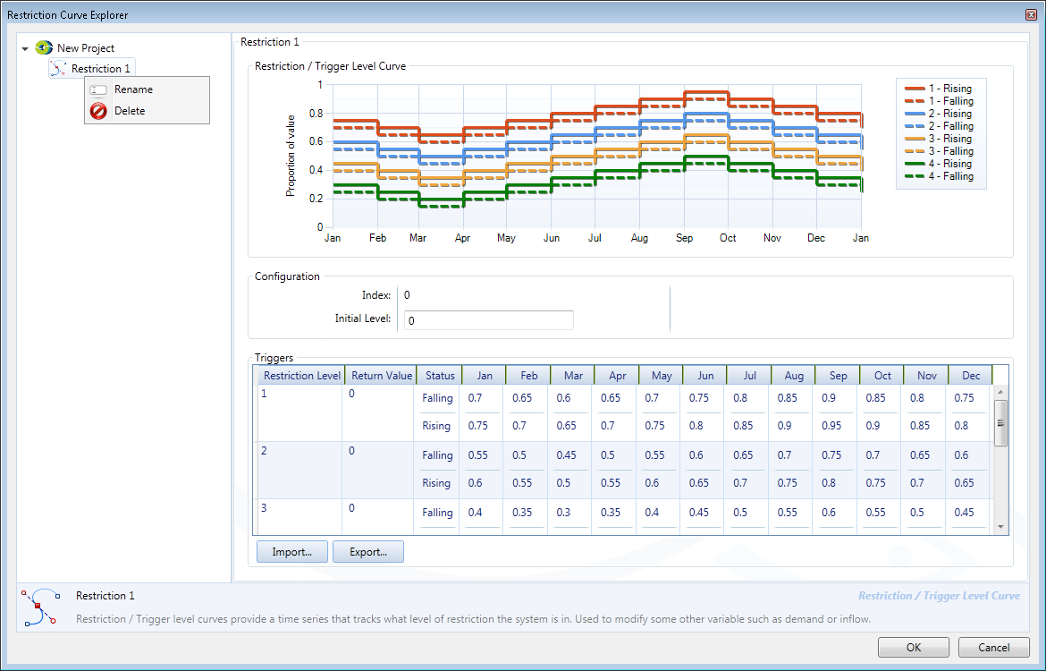
As shown in Figure 1, trigger/restriction levels might have different values depending on whether the system is rising (denotes a filling system) or falling (a falling system). The number in the legend refers to the restriction level (0 for no restrictions, 1 for restriction level 1, 2 for restriction level 2 and so on).
Figure 1. Restriction Curve Explorer
Modelling Restriction Curves
You can model restrictions in Source with the Restriction Curve Explorer by choosing . Right click New Project and choose Add Restriction/Trigger Level Curve to create a new restriction curve. You can also create multiple restriction curves, each referenced by a unique auto-generated index number, named Index. The first set of restriction curves has an index of 0 and the next 1, etc. Initial Level refers to the restriction level that the system starts in. This could be very important when modelling a scenario run with a short time series. For instance, if a model run started during a drought, the initial restriction level would need to be set to reflect this.
Specify the following values in the triggers table:
- Restriction Level - what level of restrictions the model is in;
- Return level - what value to modify the system with. You can write a function through the inflow/demand expression editor (Custom Function tab) and reference the function set in the return value;
- Falling value - trigger value for entering the restriction; and
- Rising value - the value for exiting restrictions.
You can also rename or delete the restriction curve using the contextual menu.
You must define at least two sets of restriction curves so you can move between restriction levels. Each set of restriction curves can be used to trigger a different type of event. For example, one set can be used for water resources restrictions, a second set for environmental flows and a third for desalination trigger levels. Each curve is referred to by the index number.
The restriction level time series can be used to determine performance metrics and is an important result in itself. The restriction value can be used to modify system behaviour, for instance, the restriction value returned could be a proportion to modify demand with.
Importing and exporting curves
Once you have designed your restriction curve you can export this as a .xml file which can be used on other projects. This curve can then be imported into a different project to ensure consistency and reduce set up time. Use the Export and Import buttons respectively.
To delete a restriction curve, click on the Restriction Level (in the Triggers table) that you wish to delete and press Delete on your keyboard.
