You can extend the capabilities of Source’ by adding data processing tools. Some of these "plugin" tools extend Source’ user interface, or add additional steps to the Geographic Wizard. Other plugins, especially those written by third parties, may look and operate differently from the normal user interface.

When installing plugins in Source, you must have administrator access on your computer. Some plugins are installed automatically, whereas others are placed into the plugins folder (C:\Program Files\eWater\Source\Plugins). They are files which have a .DLL or .EXE extension, and work with specific versions of Source.

Many of the existing eWater CRC Toolkit tools (or components of these tools) can be used as Source plugins; however, you must ensure that the plugin version is compatible with the Source version. For further information, ask a question via the Source support forum, at www.toolkit.net.au.

Note Ensure that there are no projects prior to loading plugins. Additionally, at times, Source might close prematurely when a plugin has been installed. Refer to Plugins related for more information.

To load a new plugin:

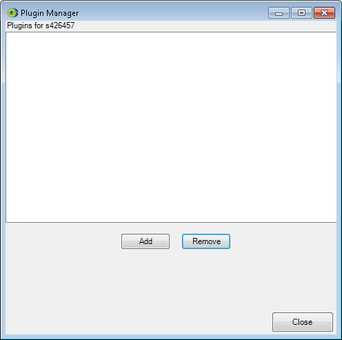
• Choose Tools > Plugin Manager to open the Plugin manager (Figure 190);
• Click Add and in the plugins folder (usually C:\Program Files\eWater\Source version\Plugins), select the plugin and click Open; and
• Click Close.

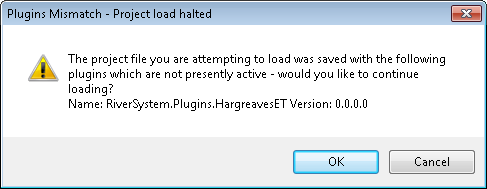
Note that if a plugin is required to run the project, but not loaded, an error appears asking if you want to keep loading the project without loading the plugin first. If the plugin is important to the project, Source might have problems running. The error tells you the name of the plugin that was used. An example of this is shown in Figure 191, indicating that the HargreavesET plugin is missing.

The following section describes the Source processing tools and component models that are installed by default. For detailed descriptions of component models, see the Source Scientific Reference Guide.

Mapping Analysis window

The mapping analysis window displays a spatial map of the constituent loads per sub-catchment and can be accessed using Tools > Analysis Windows > Map...

• In the Map Details section Runs drop-down menu, select a scenario;
• Select a variable and statistic from the drop-down menus;
• The Mapping window displays the total loads for the selected constituent in each sub-catchment; and
• Move the mouse curser over a sub-catchment in the map view. A small "tool-tip" displays near the mouse cursor, and indicates the amount of constituent exported for that sub-catchment per year (Figure 192).

You can compare statistics of two scenario runs:

• Tick the Subtract checkbox.
• Select a second scenario run in the Run drop-down menu in the section headed "Subtract".
• Select a variable and statistic from the drop-down menus.

The Mapping window displays the difference in total loads for the selected constituent for each sub-catchment in kg per year.

To display results per unit area, enable the Divide by Area checkbox.

Data unit converter

This tool converts units (embedded into data files) in Source from one unit type to another. You can access it from Tools > Analysis Windows > Data Unit Converter (Figure 193).

Use the converter as follows:

• Drag and drop the input data file onto the Source data window in the left side panel. If there are units in the data file, they should (but usually don’t) appear in the units field below the input window;
• Enter the output/target units into the Units field on the right side (under Converted Data). You can either use the default name (copied from the source data file) or enter a new name; and
• Click Convert. To save the converted file, you have to drag it somewhere else in Source that has a Save as function. You cannot right-click the converted data graph and save it.

Note that if there are no units in the input file, you must force the data converter to assume that there are input units by ticking the Override input units checkbox and entering the "assumed" unit under Units. For example, you have a CSV file containing dates and rainfall, but it does not contain any units. You want an output containing metres per day. Assume the input is in mm/day:

• Drop the input file into the Source data window;
• Tick the Override units checkbox;
• Enter mm.day-1 into the Units field;
• In the converted data window, enter the name for the converted data set;
• In the converted data window units field, enter m.day-1 (this is metres per day); and
• Click Convert. The converted data should be scaled down.

You can also scale the converted output to your desired units by ticking the Use converting quantity checkbox. Enter a non-zero value into the Value field and click Convert to scale the output by both the value and the difference in magnitude of the units eg 0.5 mm/h converted to m/h with value 3 ends up being 0.0005 m/h. Note that you must specify both the source value and the target units.

Data calculator

The Data calculator can be used to analyse spatial data and time series through the use of simple arithmetic operators. A single data set or two comparable data sets can be analysed using the data calculator. In Source, you can access it using Tools > Data Calculator.

Operations

You can use rasters, time series or numbers as operands:

• Drag and drop raster data or time series into either of the two view controls (raster or time series are displayed in a small window called a View Control (Figure 194) or use a combination of a raster/time series and a number.
• Use the radio buttons to select either the view control or the numeric value as left and right operands.
• Click one of the basic operations buttons (addition, subtraction, square root etc). The data calculator displays the operand you selected.
• Click "=", and the result, either raster/time series or numeric, appears in the results area on the right.

Note Time series and spatial data need to be in a format compatible with Source. See File formats.

Using the data calculator memory

The memory feature allows you save previous results, either numeric or raster/time series.

Click Memory to open the memory area. To save a result raster/time series into the memory, click on the 1st or 2nd operand, or result, view control, then drag and drop the contents into whichever memory view control you wish. The label above each view control shows the mathematical operation leading to the result stored there. Figure 195 shows the memory area with several stored results.

Note When you close the data calculator, the stored results are not saved. If you want to keep any of the rasters, right-click the raster, and select Save from the pop-up menu.

To save any of the results, right-click any of the view controls, and select Save from the pop-up menu. You can also drag the contents of any view control into any other view control or graph form anywhere else in Source.

The Stats tab gives a statistical summary of the data sets that have been analysed with the Data Calculator.

The Reflected Operations tab provides additional data manipulation operations, such as "Merge" data, find "Maximum value" or multiply two rasters.

Data modification tool

This functionality is yet to be documented. If you would like assistance, please call 1300-5-WATER (1300-592-837).

River Analysis Package

The River Analysis Package (RAP) contains a suite of tools for analysing the hydrology and hydraulics of a river and their relationship to ecology (Stewardson and Marsh, 2004). This section contains a summary of the tools within RAP. Most of the RAP tools can be integrated with Source through the Plugin Manager.

Location in Source: Tools > Plugins > Ecology.RAP > name of RAP tool.

The stand-alone RAP tools and accompanying user guides are available from www.toolkit.net.au/RAP.

Hydraulic Analysis module

The Hydraulic Analysis (HA) module of the River Analysis Package (RAP) is based on the Flow Events Method (Stewardson and Gippel, 2003) of allocating environmental flows. The HA module allows users to construct a one dimensional hydraulic model of a river reach and to determine ecologically-relevant flow thresholds based on hydraulic parameters such as water depth and velocity.

Plugin file: C:\Program Files\eWater\Source version\Plugins\Ecology.RAP.HA.dll

Location in Source: Tools > Plugins > Ecology.RAP.HA > name of RAP tool

HA allows you to create a time series of potentially ecologically relevant hydraulic data for subsequent analysis in TSA (Time series Analysis module) and comparison with biological data or alternative flow regimes.

HA can import HECRAS (US Army Corp of Engineers - USACE) cross-section data, as well as user input cross-section data, to create a 1-D hydraulic model of a river reach. The FldWav (pronounced "Flood Wave") (USA National Weather Service) 1-D hydraulic model is used to calculate hydraulic parameters in the reach for multiple alternative discharges.

The hydraulic parameters are presented as a rating curve for each of the hydraulic parameters versus discharge - a time series of discharge can then be converted to a time series of hydraulic parameters for analysis using RAP’s Time Series Analysis module.

HA uses channel cross-sectional data to create a one-dimensional hydraulic model. To run the 1-D hydraulic model, you must assign channel roughness factors for each cross-section. The channel roughness (Manning’s n) can be varied according to discharge, or set as a constant value for all discharges.

The main output from the hydraulic analysis module is a time series of hydraulic parameters.

Time Series Analysis module

The Time Series Analysis (TSA) module of the River Analysis Package (RAP) allows users to investigate time series.

Plugin file: C:\Program Files\eWater\Source version\Plugins\Ecology.RAP.TSA.dll

Location in Source: Tools > Plugins > Ecology.RAP.TSA > name of RAP tool

TSA is designed for use as an interpretive tool. TSA input must be daily time series, as it is designed for stream flow data, but can equally be used for hydraulic time series or meteorological data. The algorithms underlying TSA are used by the Rules Based Models (RBM) module and Quantitative Models (QM) module of RAP to predict biological responses to alternate flow scenarios.

TSA calculates time-series metrics for post-processing in other statistical packages as well as providing a graphical display of how alternative metrics change through time. TSA calculates the following time-series metrics:

• General statistics, Mean, median, Q90, Q10, Skew, coefficient of variation;
• High and low flow spell analysis;
• Colwell’s statistics;
• Rates of rise and fall;
• Base flow analysis;
• Partial series flood frequency; and
• Annual series flood frequency.

TSA has the following graphical output features:

• Display input data;
• Display graphical interpretation of time-series metrics (based on annual, seasonal, monthly basis);
• Flow duration curves (whole period, annual, seasonal, monthly);
• Flood Frequency curves (partial and annual series); and
• Base flow component of flow.

TSA allows simple drag-and-drop of common formats of daily stream flow data:

• Comma delimited (.CSV) with the first column a daily time step date and subsequent column(s) as data; and
• IQQM-standard output format from the Integrated Quality, Quantity Model produced by the New South Wales Department of Land and water Conservation.

See File formats for more information.

The basic time unit of TSA is daily, however sub-daily, monthly, seasonal and annual time series can also be handled by TSA. Time series must be gap-free (ie no empty cells if viewed in a spreadsheet).

As well as a visual output, TSA provides tabulated numeric output that can be saved as a comma-delimited file for input into other post processing statistical packages.

Time Series Manager

The Time series Manager (TSM) is a tool for manipulating, infilling, cleaning and transforming time series. It can also apply any rating curve to a time series to create new time-series data sets.

Plugin file: C:\Program Files\eWater\Source version\Plugins\Ecology.RAP.TSM.dll

Location in Source: Tools > Plugins > Ecology.RAP.TSM > name of RAP tool

The TSM module interacts with the other three components of RAP, and can:

Accept the rating curves developed in the Hydraulic Analysis (HA) module and apply them to time series; and

• Input time series to the Time series Analysis (TSA) module.

TSM allows users to investigate time series. It is intended that TSM is used as an interpretive tool and is ideal for workshop or seminar-like situations, as well as standard desktop analysis.

TSA handles most common time series formats such as *.CSV, *.CDT, *.IQQM and *.SILO8. Time series must be gap-free and be free of null entries (ie -9999).

The rating curves can be saved as .xml, which can be opened and viewed in MS Excel. Time series of hydraulic metrics can be saved as .CSV or .CDT (comma delimited time series). Bit-maps of plots can also be copied and pasted into graphics programs.

Contributor

The Contributor plugin is used to determine the amounts of a constituent that travels to a point in a network. For example, you may calculate the amount of suspended solids that runoff a sub-catchment which has been transported to the mouth of a river (as we assume proportions of the runoff are deposited in the network as it travels through the catchment).

Plugin file: C:\Program Files\eWater\Source version\Plugins\RiverSystem.Plugins.Contributor.dll

Location in Source: Tools > Plugins > Contributor > Contributor

You must have a scenario open with runs recorded before you can use Contributor.

Basic operation

Select the run and constituent of interest (functional units cannot be chosen yet).

The map will provide a graphic of the amounts of the constituent that has been contributed to the terminal (or outlet) node in the network (Figure 197). You can select another point in the system by clicking on the link above the desired node on the map. The results are automatically recalculated. The results may be standardised for catchment areas by clicking the checkbox at the bottom left of the plugin window.

The table tab shows the results in tabular form (Figure 198). You can export the results to a .CSV file by clicking Export.

Spatial data pre-processor

The spatial data pre-processor offers a range of tools that were available with the EMSS modelling framework, the forerunner of Source.

Plugin file:

C:\Program Files\eWater\Source version\Plugins\RiverSystem.Plugins.SpatialDataPreProcessor.dll

Location in Source: Tools > Plugins > RiverSystem.Plugins.SpatialDataPreProcessor

Note The Spatial Data Pre-processor plugin contains many tools that are experimental and not fully documented. The Spatial Data Pre-processor plugin will eventually be split into tools that will be built-in to Source and tools available from the Plugin Manager.

QuickRemap

The QuickRemap tool allows the grid codes to be changed in an easy manner by changing the values in the table and running the tool to get a new raster.

• Drag and drop a raster into the "src" box. This is the source raster from which the remapping will be done
• Enter the modified grid codes that map to certain layers within the raster. For example, a forest layer in a land use map may have a grid code of 3. If a scenario is required where the forest is cleared for horticulture, the grid code may need to be changed to 5, to signify that it is a Horticulture FU.
• Click the Run button and the remapped raster appears in the "dest" box. This can be saved to disk.

CreateMask

The CreateMask tool creates a new raster of the same dimensions as the sources raster with grid cell values that equal the mask value. Therefore, all non-null values in the raster grid are replaced with the maskValue parameter.

• Drag and drop a raster into the "src" pane. This is the source raster from which the remapping will be done;
• Enter a value for maskValue, which will replace all the non-null values in the raster grid. For example, a maskValue of 1 (default) will produce a new raster with the value of 1 in all cells that are not null values; and
• Click the Run button and the new mask raster appears in the "dest" pane. This can be saved to disk.

CookieCut

The CookieCut tool allows a portion of a larger raster to be "cut out" and a new raster produced. This may be useful when you only need a small segment of a large land use or DEM file.

• drag and drop the raster that a segment is to be "cut" from into the "dough" pane;
• In the cutter pane drag and drop the raster that will mark the dimensions or border of the new raster; and
• Click Run and the new segment raster is displayed in the cookie pane and can be saved using the Save icon to the left of the Cookie pane.

SelectColumns FromVectors

The SelectColumnsFromVectors tool extracts a particular attribute column from a vector map (ie shape file) and creates a new vector map based on the selected attribute.

1. Drag and drop a vector file (eg a shape file) into the sourceData pane. A list of attributes is displayed. To display the spatial extent of the attribute, select the attribute name in the sourceData pane. The number of the attribute column is displayed under Hide.
2. Set the attribute column number in the entryToTake box. In the example below a value of 1 corresponds to the GRIDCODE attribute column.
3. Click Run. The resulting vector map is displayed in the destinationData window, which contains only the attribute in the column corresponding to the value specified in entryToTake.

Sub-catchment Union

The Sub-catchmentUnion tool joins all sub-catchments in a sub-catchment raster into a single catchment area:

1. Drag and drop a sub-catchment raster into the "src" pane.
2. Click Run. The resulting catchment raster is displayed in the dest pane and can be saved by clicking Save.

HazardMap Scaling

Hazard maps are useful for informing catchment and land managers of those parts of the landscape that are most vulnerable to certain environment hazards, such as soil erosion or salinity. Scaling the Event Mean Concentration (EMC) and the Dry Weather Concentration (DWC) values using an erosion Hazard Map allows areas with "hazardous" land uses (eg highly grazed areas can be susceptible to higher levels of soil loss) to reflect the expected constituent magnitudes in such areas.

EMC and DWC parameters are determined from analysis of water quality data and are given as a minimum, median and maximum for each land use - but can be considered to apply to that land use only if it has a median erosion hazard. If the erosion hazard is above or below the median, the DWC and EMC need to be modified for that land use in that particular location. The erosion hazard map is defined as a weighted sum of the Universal Soil Loss Equation (USLE) and gully density maps (these can be generated using eWater SedNet). The weights are chosen by the user but are conceptually a function of the sediment delivery ratio (SDR). The default values are 1.5 and 0.05 for gully density and USLE respectively.

The erosion hazard map is used to compute the median, min and max values for each land use across the whole catchment, and for each land use within each sub-catchment. So, for every sub-catchment and every land use within each sub-catchment, there is a value of min, median and max erosion hazard.

The EMC and DWC values applied to a particular land use in a particular sub-catchment is computed from the ratio of sub-catchment to global values multiplied by the global EMCs and DWCs for each land use. This can be best illustrated via the hypothetical example where Table 109 for tree and grass EMCs for each sub-catchment is computed by using Table 106 and Table 107 to linearly scale Table 108.

The basic approach to scaling EMC and DWC values using a hazard map is as follows:

• Select Configure > Constituent Models > Parameters...
• Select the Scale EMCs and DWCs using Hazard Map option from the Available Methods drop-down menu.
• The sub-catchment and functional unit maps will automatically be displayed in the second and third boxes with the hazard map box initially blank.
• Drag and drop a hazard map into the blank window.

Note It is recommended that the Hazard Map be generated external to Source using a spatial data mapping and editing package.

• Select the Parameter tab. The Output, Constraint and State tabs can be ignored, as they are automatically generated by Source.
• Select the Constituent type from the Select Element drop-down menu (eg TSS).
• Manually enter or load in a text file containing functional unit name, minimum median and maximum EMC values for each corresponding functional unit type. An example is given in Figure 205 for EMC values. Repeat for DWC window.

Note Functional unit names must exactly match the list displayed in the EMC window. An alternative approach is to save out the empty EMC/DWC files as a template to ensure functional unit names/spaces and spelling are correct. This table can then be populated with minimum, median and maximum EMC/DWC values and loaded into Source.

• Percentile - specifies the percentile bound for generating the regional hazard statistics visible under the State tab;
• Processing cell size - this parameter can be ignored. The ProcessingCellSize is used when rasterising the FU land use and Hazard maps, and is set to a default of 100, which is 100 meters wide (and high). A smaller the size results in a finer the scale for spatial scaling of erosion hazard values, but processing will take longer; and
• Use FU areas - this parameter can be ignored as it is automatically generated and requires no input from the user.
• Click Run;
• When processing is complete the green progress bar at the bottom of the screen will have moved across;
• If more than one constituent type is listed, then a new constituent will need to be selected from the drop down list at the top of the screen. A new set of corresponding EMC/DWC values need to be loaded to correspond to the new constituent selected; and
• Select Close when appropriate EMC/DWC values have been assigned for all constituents.

StreamOrder Lengths

The StreamOrderLengths tool gives a summary of the lengths (in meters) of the river reaches and streams for each sub-catchment so that management tasks, such as riparian buffer zones, can be applied to specific stream orders within sub-catchments.

Select Tools > Plugins > RiverSystems.Plugins.SpatialDataPreProcessor > StreamOrderLengths. The Stream Order Lengths window appears:

• Drag and drop a stream order raster into the StreamOrderRaster pane;
• Drag and drop the sub-catchment map into the Sub Catchment Raster pane;
• Adjust the sinuosity factor if necessary (default value is 1.25);
• Click Create to create a table summarising the stream orders and lengths per sub-catchment; and
• Click Save to save the table. Source saves this as a tab-delimited file (.txt).

ExtractRaster

The ExtractRaster tool allows a spatial layer to be extracted from a raster. Therefore, if grid code 3 is entered in the "val" box, then all grid codes referenced as 3 will be extracted from the source raster (src).

• Drag and drop a raster to the "src" box;
• Enter the grid code value of the layer that is to be extracted; and
• Click the Run button. The extracted raster is displayed in the "dest" box.

Catchment import tool

This tool allows you to manually define a catchment network with a large number of sub-catchments. It is accessed from step 3 of the Geographic Wizard, under the method "Draw Network".

Under the button to open a catchment file "Load Sub-catchment Map" you’ll find a checkbox and two buttons if this tool in enabled for your version of Source.

In summary, the import links tool has three modes of operation:

• Confirm each link before committing it to the list of links by checking the Confirm each link checkbox. This ensures that you verify each link before it is created and added to the database of links;
• Import a shape file of proposed links using Load Background Map. This aids in tracing the network and displays an existing file of links, which can be used to create links in a GIS format. This can then be exported to a shape file, using the catchment map and its surroundings as a background. Finally, this file can be superimposed onto the sub-catchment map to "click" on the right locations; and
• Select Add links Shp file to ensure that Source reads directly from a shape file to create valid links.

PERFECT GWLag Plugin

This plugin allows you to model groundwater and its interactions in a sub-catchment. To use the groundwater tools in Source, ensure that the following plugin has been installed:

RiverSystem.Plugins.PerfectGWLag.dll

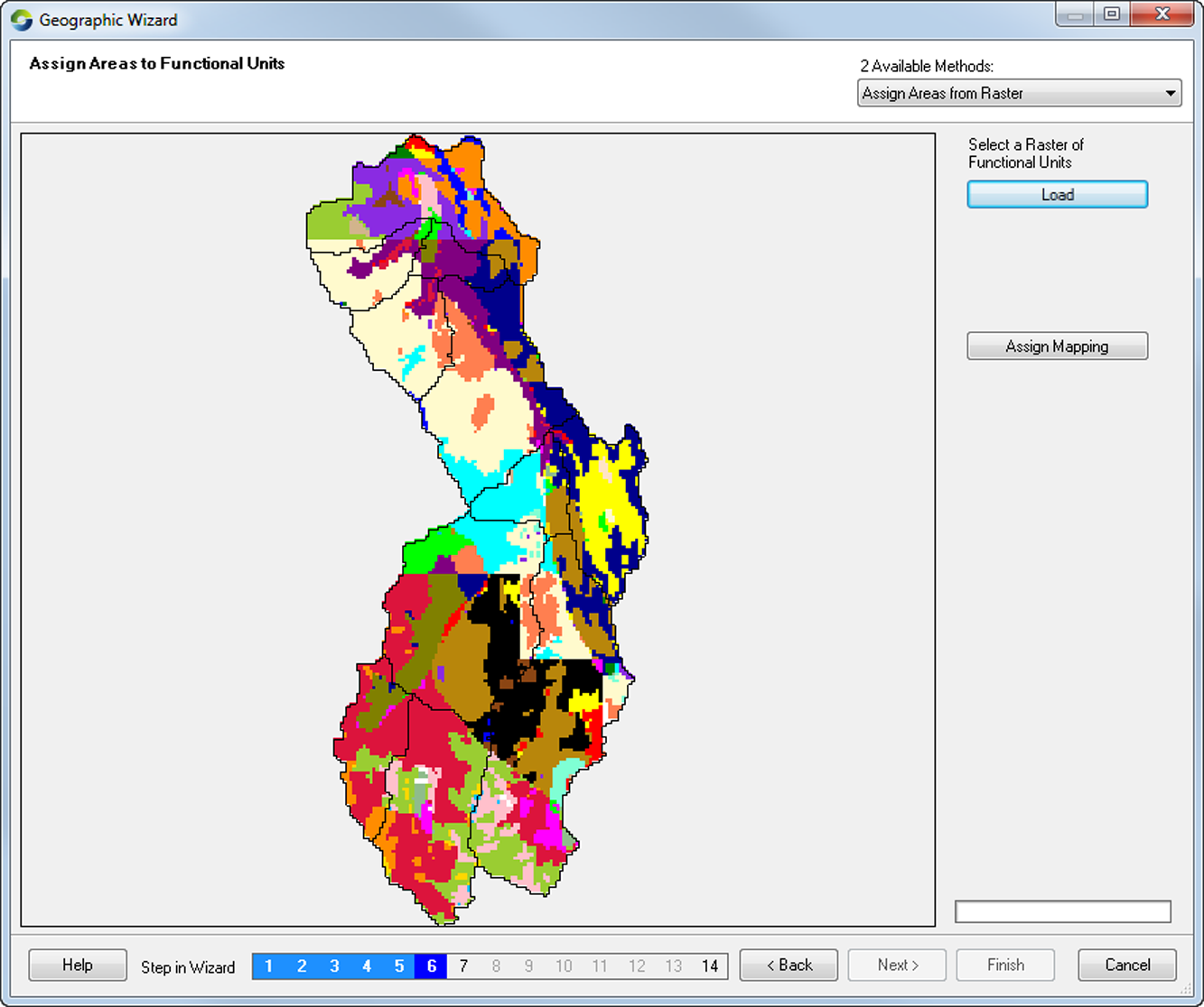
The next steps involve creating a sub-catchments scenario with the Geographic Wizard for catchments, and configuring various parameters to model groundwater. Just as with any catchments scenario, use the wizard to first create a standard set of sub-catchments to suit your study area and modelling requirements in Define the network (Step 3). Next define the functional units using a shape file (refer to Specify functional units (Step 5) for details) and assign areas to them using a raster (Specify functional unit areas (Step 6)). Figure 209 shows an example of this. The next section provides details on configuring rainfall runoff, constituent generation and filter models in Source.

Defining and assigning models

You can then assign models to rainfall runoff, constituent generation, and any filtering you wish to the sub-catchments using the wizard or the options in the Edit menu (refer to Rainfall runoff models and Constituent generation and filtering models for details):

• Constituent generation - add "Salt" as a constituent and assign the "Simple GW salt model";
• Rainfall runoff - assign "PERFECT GWLag" as a model. To assign inputs, choose PERFECT GWLag model input assignment from the Available Methods drop down menu (Figure 210) and load the weather database you wish to use. Check the following:
• the station number from each FU (left hand column) match the station numbers on the right hand side (drop down lists, right hand columns). If they do not, the entry on the right hand side will be the closest text based match, not the closest geographic match. You can adjust the matches by selecting an alternate station from the drop down list of stations available in the loaded weather database; and
• Note that the minimum and maximum dates will be displayed by default. To save memory you can either import the desired time period or import the entire range but run the model for a selected period. The latter is a more flexible option.
• Filter - Assign any filter model you wish from the drop down menu;
• Links - you can add a model to selected links and if flow routing or a storage model is required. Note that there is no link model specific to the Groundwater tools in Source; and
• Nodes - select FlowScaledLossModel from the Node models drop down list and click Add Model.

Parameterising models

This section describes how to parameterise each of the assigned models. It requires the parameterisation of both components - PERFECT and GWLag.

Rainfall runoff

Choose PERFECT-GWLag model parameterisation" from the Available Methods drop down list. The PERFECT and GWLag parameters are specified under separate tabs.

To parameterise PERFECT:

• Select the Landuse tab under Perfect Parameters and click Load. Import the land use database in the same way as for the weather database;
• Once the database is loaded, check and adjust the crop and soil parameter associations. You may also choose to set the initial conditions such as "Proportion of Field Capacity" or "Crop Residue"; and
• Select the Soil tab under Perfect Parameters and click Load. Repeat the process for land use by loading a soils database for specifying soil association groups.

Figure 211 shows an example of this.

To parameterise the GW Lag components, click on the Lag GW parameters tab (shown in Figure 212):

• Set all the global parameters; these can either be changed individually or all at once. To set individually click on the appropriate cell and type a new value. To make changes to all values in a column (e.g. one parameter) change one cell to the desired value. Next right-click in a cell either above or below (in the same column) and select Apply to all sub-catchments from the contextual menu;
• Specify the groundwater parameters by importing them from a GFS shape file. Click Load in the Ground Flow System parameters group box and load a GFS shape file;
• Next, match the fields for aquifer thickness, hydraulic conductivity and storativity from the loaded GFS shape file by selecting the appropriate field name from each of the three drop-down lists; and
• Click Apply.

Constituent generation

Choose SimpleGWSaltModel parameterisation from the Available Methods drop down list (Figure 213).

• Specify the through flow salinity percentage value using the up/down arrows;
• Specify rainfall salinity by loading a rainfall salinity raster, or enter a single value;
• Enter the averaged aquifer salinity by loading a GFS shape file in the Groundwater Flow System parameters group box; and
• Choose the field name that represents aquifer salinity using the drop down menu and click Apply.

Node

Select the node from the list of node models and click Configure. The resulting window (Figure 214) shows the parameters that can be changed.

Groundwater pumping

You can also attach catchment scale models to the required sub-catchments by clicking on a sub-catchment and selecting Groundwater Pumping Model in the Catchment Models drop down menu. Click Add Model and select the required pumping model. Click Parameterise to open Figure 215.

To parameterise the groundwater pumping model, you need to have at least one pump. This can be done either manually or by importing a shape file. To add one manually, ensure that AddSingle is present in the Add Method drop down menu and click Add. The properties for the new pump will be displayed below. Any properties that appear in bold text (such as Name) can be changed. Clicking on these will result in an ellipsis appearing, which must be clicked to make changes.

If you have more than one pump added you can switch between them by selecting the desired pump under Pumps on the top left hand side. When first added, each new pump will have a default value for DistanceProperties, which can be set by clicking on PumpingRiverImpact.

The default values for distance are:

• DistanceToImpactLocal: The distance between the sub-catchment centroid and the outlet;
• DistanceToImpactRegional: The distance between the sub-catchment centroid and the scenario outlet i.e. the outlet of the most downstream sub-catchment in the scenario; and

• A new dialog will appear that allows you to change either the local or regional impact distance. To enter a new value for either click in the NumericUpdown box and change the current value to the desired one. When finished click "Apply".
• By default no values are set for the "gfsProperties" aquifer thickness, storativity, and hydraulic conductivity. When set these groundwater properties are used to set the diffusivity of the aquifer the pump is installed in.
• "gfsProperties" can be set by clicking on the property value "PumpingRiverImpact. gfsProperties" which is highlighted in bold text. Once clicked on a small box will appear with 3 dots in it, to the right of the property name, click on the small box to set (Figure 216).

• A new dialog will appear that allows you to either set the value for each property manually or estimate them using s GFS shape file (#anchor-38-anchor).
• To adjust the GFS properties manually, click on the desired up or down arrows to the right of the field and press "Apply".
• To set the properties using a GFS shape file;
• Click on the "Load" button and select a GFS shape file
• Next click on each of the three combo-boxes and match the field name from the shape file to the GFS property name next to the combo-box (Aquifer thickness, Hydraulic conductivity, Storativity (#anchor-39-anchor).
• When all three values are set, press the "Import" button.
• Then press the "Apply" button.
• Each pump can have one or more Pumping Instance, which is a period of extraction at a certain rate. By default a single Pumping Instance is added for each new pump. Pumping Instances appear on the right hand side of the form in the in the "Pumping Instance" group box. To view and set the properties of a pumping instance click on it in the list box on the top right hand side of the form, the properties for each instance appear below. You can set any properties in bold. Valid values for StartDate, EndDate, PumpingRate, and RegionalImpact should be set by clicking on the property name which is highlighted in bold text. Once clicked on a small box will appear with 3 dots in it, to the right of the property name, click on the small box to set. The property RegionalImpact should be set to true if the impact is to be applied at end of catchment and left as false in all other cases.
• Additional PumpingInstances can be added by clicking on the "Add" button to the right of the PumpingInstance list box (#anchor-35-anchor). Likewise existing ones can also be removed by clicking the remove button.
• Once the pumping configuration has been completed, click Apply

The GWlag global parameters can be changed via:

Any of the added rainfall runoff, constituent generation or filer model parameters can be changed through the Edit menu.

Writing your own plugins

When you install Source, instructions for writing your own plugins are included along with a series of templates to help you get started. Under Windows XP, the standard location is:

C:\Program Files\Source n.n.n.n\Plugins\ExamplePlugins.zip

Under Windows 7, the standard location is:

C:\Program Files\eWater\Source n.n.n.n\Plugins\ExamplePlugins.zip

where n.n.n.n is the version number of Source. If you boot Windows from a different hard disk drive or have otherwise customised your installation, you should make the necessary adjustments.

Please consult with your system administrator if local security policies prevent you from accessing this package.