Function manager
- Geoff Davis
- asatheesh (Unlicensed)
- mah135 (Unlicensed)
- Former user (Deleted)
Functions
A component's behaviour can depend on other dynamic values within a model. Functions allow you to control this behaviour via an arithmetic expression, or function.
About the Function manager
The Function manager (shown in Figure 1) allows you to centrally manage all functions that have been defined in Source. It is used in places where you might otherwise employ a time series or a single value.
The Function manager can be accessed in one of two ways:
- Choosing View » Function Manager; or
- Clicking on the Function Manager icon in the Scenario toolbar.
Figure 1. Function manager
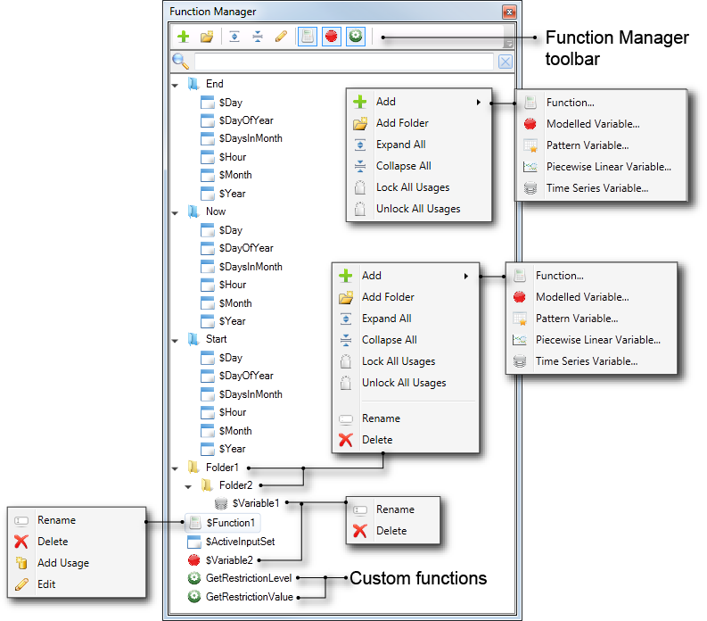
Items in the Function manager are sorted into groups, and then by name. Groups are ordered as follows:
- Folders associated with In-built variables, which includes End, Now, Start;
- Functions;
- Variables - there are four types of variables available in Source. Refer to Types of variables for more information; and
- Custom functions.
Usages
When a function is used in the model, as an example at an inflow node, then that usage is shown in the tree under the function. If a function is used in multiple places, then all usages are shown under the function in the Function Manager tree. To link a node to a function, you can either:
- Use the node's feature editor; or
- Right click the function and choose Add Usage. Then, use the Metaparameter Explorer.
The Function Manager only shows direct uses of a function. For example, if an inflow node has been assigned a function, $ExampleFunction, this is indicated in the Function Manager. If $ExampleFunction is comprised of two separate functions, $ExFn1 and $ExFn2, these two functions will not be part of the Inflow node.
You can also search for a variable or function using the area under the Function manager toolbar. Start entering the search item, and the results will be filtered as you type the text.
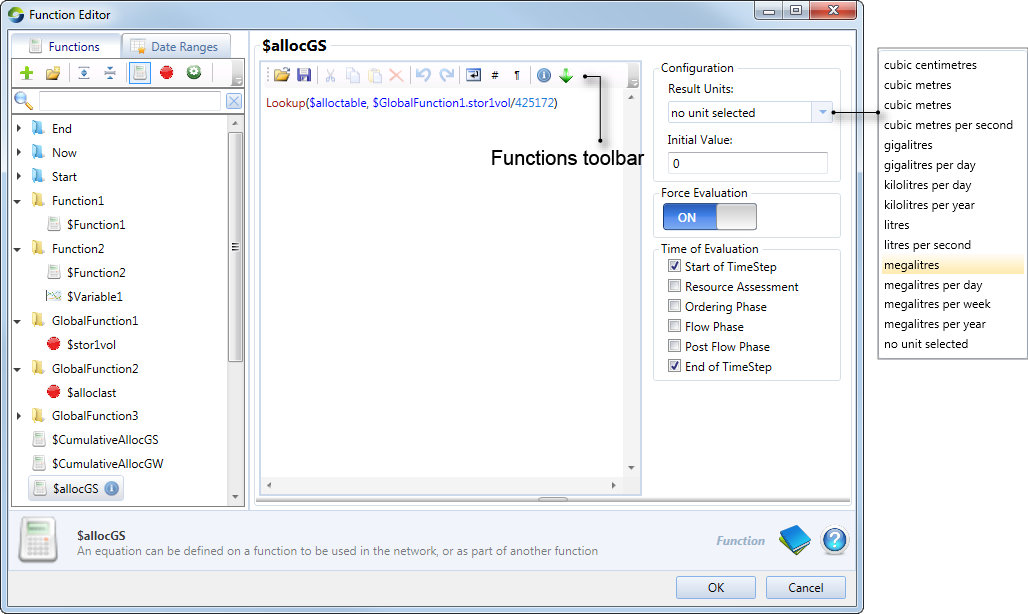
Function Editor
The Function Editor (shown in Figure 3) allows you to add, modify and delete individual functions and variables. It can be accessed in one of two ways:
- Choosing Edit » Functions…; or
- Choose the variable you want to change in the Function manager (Figure 1). Right click on it, then choose Edit from the contextual menu.
Figure 3. Function Editor
Adding a variable or function
To add a variable or function, click on the Add Variable button on the Functions toolbar (as shown in Figure 1) and choose the appropriate drop-down item;
You can define and configure it using the Configuration pane on the right. The view of this pane will depend on the type of variable or function that has been specified.
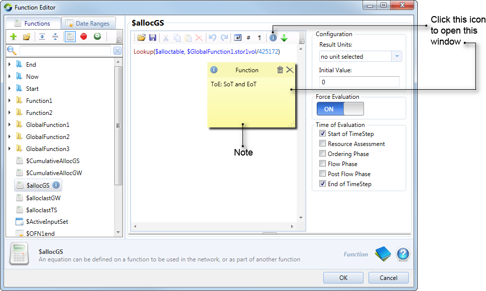
Adding a note to a function
You can include a text-based message, or note, to be associated with a function. Refer to About notes for more information about notes.
To associate a note with a function (as shown in Figure 4):
- Open the Function Editor;
- Click on the function you want to add a note to;
- In the Function Editor toolbar, click on the Add/Edit Note icon; and
- Add the text message in the window that appears.
Figure 4. Function Editor, Adding a note
Deleting and renaming a variable or function
To delete a variable or function, choose the appropriate item in the function list, right click, and choose Delete from the contextual menu.
To rename it, choose Rename from the contextual menu and type the name you wish to assign.
The Results Units drop down menu allows you to choose which units the variable or function will evaluate to. The result units of a function have to commensurate to the required units of the model input it is used for. If the result units of the function aren't the same as the required units of the model input, a conversion is done of the function result before it passes the value to the model.
By default, if a function is not referenced at any model input, or any other functions, it is not evaluated during a scenario run. The Force Evaluation scroll toggle (Figure 2) ensures that a function is evaluated during a scenario run. You would use Force Evaluation if you wanted to record a function that wasn't being used, or if you had a modeled variable pointing to a function that wasn't evaluated. The only downside to turning on Force Evaluation for all functions is that the performance will be effected.
The Initial Value for a function is only used when a function references itself. The Initial Value is in this case for the first evaluation of the function.
You can also enable recording of a function using the Project Explorer (choose Miscellaneous).
About variables and functions
General rules for functions
The following rules apply to functions:
- White-space, including new-line markers, is ignored;
- Function names, operator names, variable names and label names are not case sensitive;
- All variable names must begin with the "$" character;
- All variables used in functions must be defined;
- Functions can reference themselves. The initial value is used in this case for the first evaluation of the function.
- Circular references are prohibited between multiple functions; and
- A blank function returns zero.
Scoping
Functions and variables can have non-unique names, so long as they are in different scopes. For example, consider the following setup in the Function manager:
ANU: CAN WE USE PROPER SCREENSHOT HERE
	Folder1
		$Function1
		$Function2
	Folder2
		$Function3
	$Function4
- In this case, $Function1’s expression can reference $Function2 directly as they are both part of Folder1. So, if($Function2, 0, 1) is a valid function;
- If $Function3 references $Function2, you must use the full path to reference it - if($Folder1.Function2, 0, 1); and
- Any function can reference $Function4 directly because it is in the global scope (ie. it is not part of a folder).
There are several in-built functions and operators that allow you to define otherwise complex functions in simple expressions. These are described next.
Operator precedence
Unless you use parentheses to modify the order of evaluation, operations are performed according to the precedence rules shown in Table 1. Where two operators have the same level of precedence, the operations are performed left-to-right.
Table 1. Function manager (evaluation order)
| Order of precedence | Operator Symbol | Meaning |
|---|---|---|
| 1 (highest) | ( ) | explicit ordering |
| 2 | - | negation |
| 3 | ** and ^ | exponentiation |
| 4 | * and / | multiplication and division |
| 5 | + and - | addition and subtraction |
| 6 (lowest) | < <= = >= > <> | comparison operators |
In-built functions
In-built functions are predefined formulae that perform calculations which usually depend on the arguments you supply as parameters. They can be entered manually or by using the pull down menu at the top of the Function Editor (Figure 2). The available functions are summarised in Tables 6-10. Some examples of function use are shown in Table 2.
Table 2. Sample expressions using functions
Expression | Result | Expression | Result | Expression | Result |
|---|---|---|---|---|---|
Average($var1) | 3 | Median($var1) | 3 | Lookup($var1,13.5) | 2.5 |
Lookup($var1,14) | 3 | Count($var1) | 5 | Max($var1) | 5 |
Min($var1) | 1 | Sum($var1) | 15 | Stdev($var1) | 1.58113883 |
Where: $var1 is the piecewise linear relationship {(12, 1), (13, 2), (14, 3), (15, 4), (16, 5)}
Table 3. Function manager (arithmetic operators)
Operator | Meaning | Example | Result |
|---|---|---|---|
+ | addition | 10 + 5 | 15 |
- | subtraction; negation | 10 - 5 = 5 or 10 + (-5) | 5 |
* | multiplication | 10 * 5 | 50 |
/ | division | 10 / 5 | 2 |
** or ^ | power/exponentiation | 10**5 or 10^5 | 100000 |
( ) | influence order of evaluation | 5 * (10 + 5) | 75 |
Table 4. Function manager (comparison operators)
Operator | Meaning | Example | Result |
|---|---|---|---|
> | greater than | 10 > 5 | true |
< | less than | 10 < 5 | false |
>= | greater than or equal | 10 >= 5 | true |
<= | less than or equal | 10 <= 5 | false |
= | equal | 10 = 5 | false |
<> | not equal | 10 <> 5 | true |
Table 5. Function manager (logical operators)
Operator | Meaning | Example | Result |
|---|---|---|---|
OR | or | false OR true | true |
AND | and | false AND true | false |
NOT | not | NOT false | true |
Table 6. Function manager (general mathematical functions)
Function | Meaning | Example use |
|---|---|---|
EXP | Returns e raised to the power of a given number | EXP(number) |
LOG10 | Returns the base-10 logarithm of a number | LOG10(number) |
LN | Returns the natural logarithm of a number | LN(number) |
ABS | Returns the absolute value of a number | ABS(number) |
SQRT | Returns a positive square root | SQRT(number) |
MOD | Returns the remainder from division | MOD(number,divisor) |
ROUND | Rounds a number to the nearest integer | ROUND(number) |
INT | Rounds the number down to the nearest integer | INT(number) |
Table 7. Function manager (statistical functions)
Function | Meaning | Example use |
|---|---|---|
AVERAGE | Returns the average of its arguments | AVERAGE(variable_name) |
COUNT | Counts how many numbers are in the list of arguments | COUNT(variable_name) |
COUNTIF | Counts how many numbers in the list of arguments satisfy the expression | COUNTIF(variable_name,expression) |
MAX | Returns the maximum value in a list of arguments | MAX(variable_name) or MAX(number,number) |
MEDIAN | Returns the median of its arguments | MEDIAN(variable_name) |
MIN | Returns the minimum value in a list of arguments | MIN(variable_name) or MIN(number,number) |
STDEV | Estimates standard deviation based on a sample | STDEV(variable_name) |
SUM | Adds its arguments | SUM(variable_name) |
Table 8. Function manager (trigonometric functions)
Function | Meaning | Example use |
|---|---|---|
ARCCOS | Returns the inverse cosine of a number | ARCCOS(number) |
ARCSIN | Returns the inverse sine of a number | ARCSIN(number) |
ARCTAN | Returns the inverse tangent of a number | ARCTAN(number) |
COS | Returns the cosine of a number | COS(number) |
SIN | Returns the sine of a number | SIN(number) |
TAN | Returns the tangent of a number | TAN(number) |
Table 9. Function manager (miscellaneous functions)
Function | Meaning | Example use |
|---|---|---|
IF | Specifies a logical test to perform | IF(logical_test,value_if_true,value_if_false) |
LOOKUP | Looks up the Y-value corresponding to an X-value via a piecewise linear editor (uses linear interpolation) | LOOKUP(variable_name, number) |
N1 | Returns 1 if the number is less than zero, 0 otherwise | N1(number) |
P1 | Returns 1 if the number is greater than zero, 0 otherwise | P1(number) |
PI | Returns the mathematical constant π to 14 decimal places | PI() |
| /* Comment */ | /* begins a comment and */ ends a comment. Comments can go over multiple lines. | 5 + 4 /* Some sort of comment about the function*/ |
Table 10. Function manager (predefined variables)
Function | Meaning |
|---|---|
$Now.Year | Returns the 4-digit year of the current time-step |
$Now.Month | Returns the month of the current time-step (range: 1...12) |
$Now.Day | Returns the day of the current time-step (range: 1...31) |
$Now.Hour | Returns the hour of the current time-step (range 0...23) |
| $Now.DaysInMonth | Returns the number of days in the month for the current time-step (range, 28..31) |
| $Now.DayOfYear | Returns the current day in the year for the current time-step (range, 1, 366) |
| $Start.Year | Returns the 4-digit year of the simulation start date |
| $Start.Month | Returns the month of the start of simulation date(range: 1...12) |
| $Start.Day | Returns the day of the simulation start date (range: 1...31) |
| $Start.Hour | Returns the hour of the simulation start date (range 0...23) |
| $Start.DaysInMonth | Returns the number of days in the month for the simulation start date (range, 28..31) |
| $Start.DayOfYear | Returns the current day in the year for the simulation start date(range, 1, 366) |
| $End.Year | Returns the 4-digit year of the simulationend date |
| $End.Month | Returns the month of the simulation end date (range: 1...12) |
| $End.Day | Returns the day of the simulation end date (range: 1...31) |
| $End.Hour | Returns the hour of the simulation end date (range 0...23) |
| $End.DaysInMonth | Returns the number of days in the month for the simulation end date (range, 28..31) |
| $End.DayOfYear | Returns the current day in the year for the simulation end date (range, 1, 366) |
| $ActiveInputSet | Returns the simulation input set. Can be used in statements like if($ActiveInputSet = "Wet", 15, 10) |
Writing functions
The following features in Source are available when writing functions:
- Source has an auto-complete feature, which assist with code completion. For example, if you enter '$', a list of available choices appears, showing all the variables and functions that can be used;
- Press Ctrl + Space to view all the available keywords, such as 'min' or 'average'. These keywords can also be viewed by using the keyword button on the toolbar; and
- You can drag and drop variable names into a function.
Figure 5. Maximum Constraint node (Function Editor)
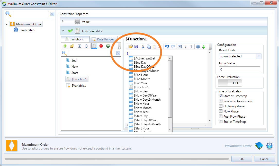
Referencing
A function can reference other functions within the same scenario. It can also reference itself.
For example: $Function1 = $Function1 + $Function2
In this case, $Function1 will use its previous evaluation value to calculate its new one.
Notice that the list shown in Figure 3 contains $Function1 as an option.
Testing Functions
Once you have defined a function, you can test its operation using the Parse button. You can enter values for the various terms in your function and confirm that the result of evaluating your function with those values is correct. The Parse button is, by default, hidden in the Function editor, and is used as follows:
- Select the function you wish to test. This will appear in the Configuration pane of the Function editor;
- Click on the area below the Configuration pane (as shown in Figure 6);
- If the variables/functions used in the function aren't in the list, click Parse
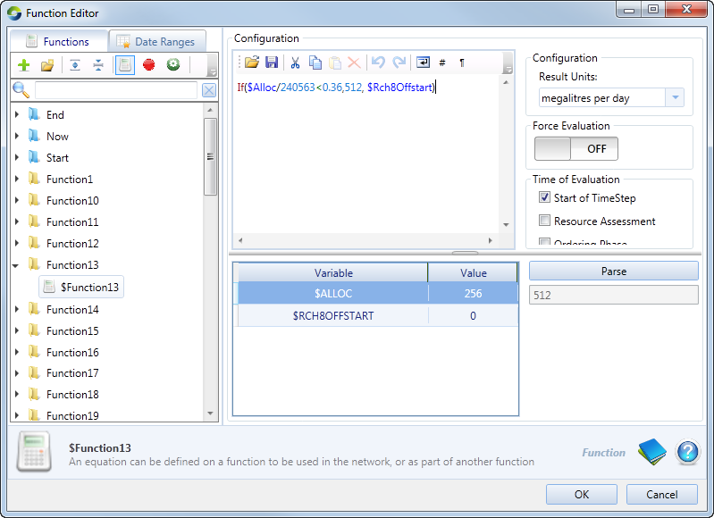
- The expanded section (shown in Figure 7) provides a table of all the variables used in the function. Enter a value for the variable you wish to test (double-click on the cell, then enter a number);
- Click Parse; and
- The test result will be displayed in the cell under the Parse button.
To close this area, click on the same position.
Figure 6. Function Editor (Parse)
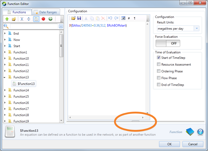
Figure 7. Function Editor (Parse-window)
If the function cannot be parsed, you will get an error icon next to the function in the Function manager. Additionally, an error in the Log Reporter will be available at run time to indicate the same.
Types of variables
Modelled variables
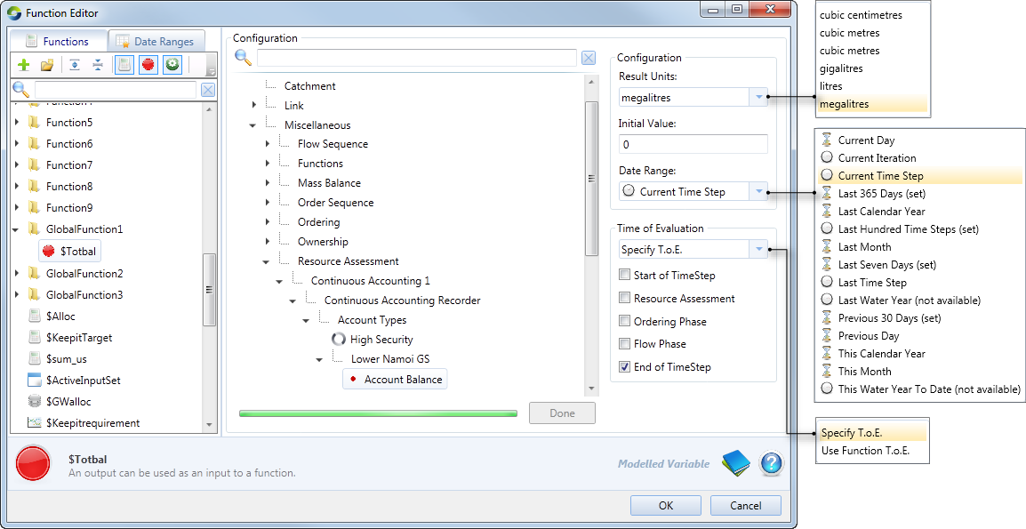
A modelled variable provides a connection between your function and model variables. You define a name (or meta-name) by which you will refer to a model variable in your function and configure other parameters governing its use. Once a variable has been defined, it can be used in a function. To configure a new modelled variable using the Function Editor:
- Add a modelled variable, as described in Adding a variable or function;
- A new variable will appear in the position that was selected. Note that at this point, the variable has not been allocated a recorder, so a warning icon will appear;
- The Configuration pane will show a list of all the recorder variables available (this will depend on the model);
- Using the disclosure triangles, choose the appropriate recorder that you wish to be associated with the variable;
- Depending on the recorder you choose, you can also specify the following:
- Result Units - units of the results;
- The variable's Initial Value - this defines the value that the variable takes on between the start of the first time-step and the point during that time-step when the corresponding model variable acquires a defined value;
- Date Range - the date range that the Function manager uses as a filter when obtaining data during each time-step. For example, you can choose to use the value from the current time-step or the previous time-step. You can also use values like the average of the last 100 time-steps. See Date ranges for more information; and
- Time of Evaluation - specifies when the variable will be evaluated. See Time of Evaluation for more information; and
Figure 8. Function manager (Variables tab)
Piecewise Linear variable
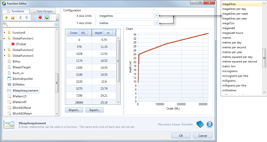
A piecewise linear variable (shown in Figure 9) allows you to create piecewise linear relationships for use in functions. You can find more information about such relations at About piecewise linear editors.
To define a new piecewise linear relationship:
- Create a new Piecewise Linear variable as described in Adding a new variable or function;
- In the Configuration pane, either import a table to assign a piecewise linear relation, or enter one manually; and
- Set the units appropriate to the X and Y axes using the appropriate drop down menus.
Refer to About piecewise linear editors for more information on constructing relations.
Figure 9. Function Editor (Piecewise Linear relation)
Patterns
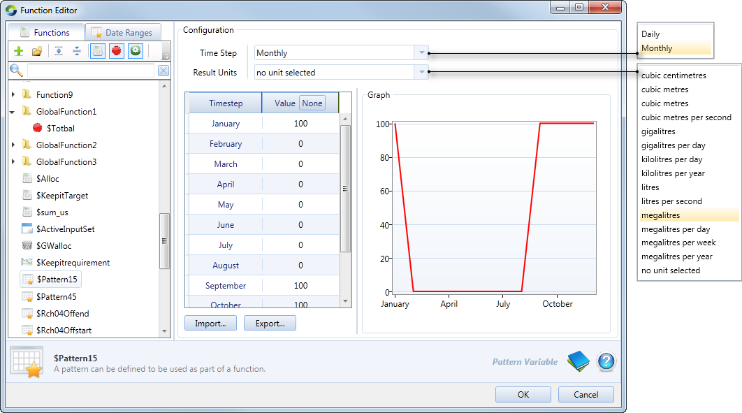
You use patterns (Figure 10) to create a named dataset of repeating time-dependent values (eg. daily or monthly pattern).
To define a new pattern variable:
- Create a new Pattern variable as described in Adding a new variable or function;
- In the Configuration pane, either manually or via a text file, enter the amount per time period specified, eg. monthly accepts 12 values ;daily accepts 366 values;
- Specify either a daily or monthly time-step; and
- The units for pattern values are the units defined for the simulation. To convert the entered data to different units for use in the functions, choose the new units from the Result Units drop-down menu.
Source evaluates the function equation for each time-step and returns a value for each time-step.
Figure 10. Function Editor (Patterns)
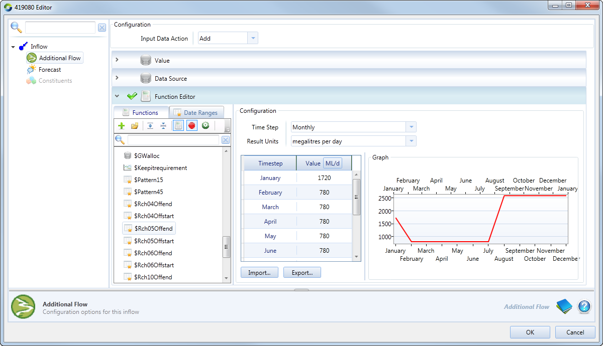
Example - Application of the Patterns variable using an inflow node as an example
As an example, the Function Editor is used in the Inflow node to specify the values of monthly inflows using a Patterns variable (Figure 11).
Example: You want to use mean monthly inflows for every time-step in a monthly model simulation.
Use Case: The inflow node is connected to the river network. In the node’s feature editor, select the Function Editor as the preferred data input method. Then, choose a function that refers to the pattern (eg. $Pattern).
Figure 11. Inflow node (Function Editor - Monthly pattern)
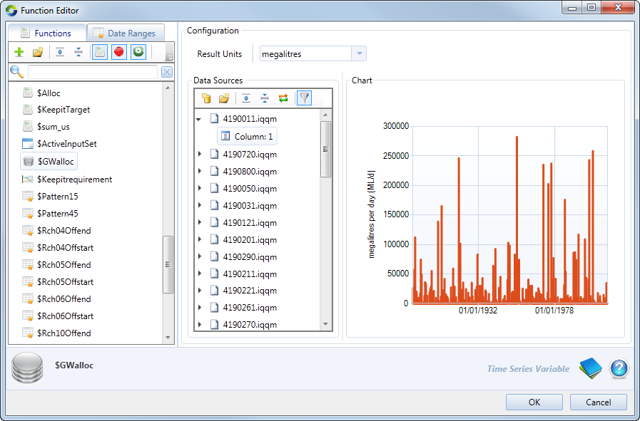
Time Series variable
You can assign a variable to use a time series as an input:
- Create a new time series variable as described in Adding a new variable or function;
- In the Configuration pane, assign a time series (using the Data Sources panel) to the variable; and
- Specify the Result Units - this will be assigned depending on the time series. The function system will convert the time series value each time step from the units of the time series, to the Result Units of the time series variable.
Figure 12 shows an example of a Time series variable. Refer to Importing data for information on working with the Data Sources panel.
Figure 12. Function Editor (Time Series variable)
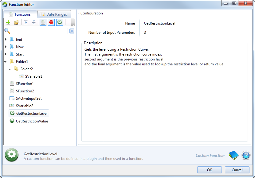
Custom Functions
Allows you to create your own expression and then import it for use in the Function manager. Refer to /wiki/spaces/SC/pages/51643422. The Parameter count column refers to the number of arguments used in the function.
Figure 13. Function Editor (Custom Functions)
Time of Evaluation
Functions are evaluated at the start of each time-step. 3.5.0 Simulation phases shows details of all phases involved in a simulation time-step:
- start of the ordering phase;
- end of the ordering phase;
- start of the flow distribution phase; or
- end of the flow distribution phase.
Date ranges
All events occurring during a time-step are independent, such as when a function is evaluated, or when the modeled variable on which the function depends is updated. You can choose the times in which to carry out certain actions. Tables 11 and 12 define the options which are available by default.
If none of the default options is appropriate, you can define your own date ranges using one of the options from the Date range type popup menu (Figure 15).
Table 11. Function manager (date range instances)
Date Range | Meaning |
|---|---|
Current Time-step | The most-recently-updated value. |
Current Iteration | Only applicable to NetLP. The value updated during the last iteration of the solver. |
Current Day | For a daily model, this is a synonym for Current Time-step. For a sub-daily model, it is the sum of the values for the current day. |
This Month | For a monthly model, this is a synonym for Current Time-step. For a sub-monthly model, it is the sum of the values for the current month. |
This Calendar Year | For a yearly model, this is a synonym for Current Time-step. For a sub-yearly model, it is the sum of the values for the current calendar year. |
This Water Year To Date | For a yearly model, this is a synonym for Current Time-step. For a sub-yearly model, it is the sum of the values for the current water year. |
Last Time-step | The value of the variable at the completion of the previous iteration of the model. |
Previous Day | For a daily model, this is a synonym for Last Time-step. For a sub-daily model, it is the sum of the values for the previous day. |
Last Month | For a monthly model, this is a synonym for Last Time-step. For a sub-monthly model, it is the sum of the values for the previous month. |
Last Calendar Year | For a yearly model, this is a synonym for Last Time-step. For a sub-yearly model, it is the sum of the values for the previous calendar year. |
Last Water Year | For a yearly model, this is a synonym for Last Time-step. For a sub-yearly model, it is the sum of the values for the previous water year. |
To calculate a particular date in the water year using the calendar date functions, you can use $now.dayofyear+184 (to indicate the next calendar year) for example, or $now.dayofyear-181 (represents the current calendar year).
Table 12. Function manager (date range sets)
Date Range | Meaning | Example of use |
|---|---|---|
Last Hundred Time-steps | The set of values from the model for the previous 100 iterations. | Lookup($var,35) |
Last Seven Days | For a daily or monthly model, this is the set of the values from the last seven time-steps. For a sub-daily model, it is the set of the average daily values for each of the previous seven days. | Average($var) |
Previous 30 Days | For a daily or monthly model, this is the set of the values from the last 30 time-steps. For a sub-daily model, it is the set of the average daily values for each of the previous 30 days. | Average($var) |
Last 365 Days | For a daily or monthly model, this is the set of the values from the last 365 time-steps. For a sub-daily model, it is the set of the average daily values for each of the previous 365 days. | Average($var) |
Custom date ranges fall into three categories:
- Date Range Calendar (Figure 13) allows you to define a precise start and end date during which the model variable is considered to be valid. Enabling the Is Recurring checkbox ignores the years. In other words, the period between [start day/start month] and [end day/end month] is valid for every year during model execution.
- Date Range Period (Figure 14) allows you to specify the date range in terms of a period of time that is relative to the current time-step. A period can range from one hour to one year and is controlled via the Period popup menu. The number of periods included in the range is controlled by the X periods ago(start) and Y periods ago(end) fields where end ≥ start. A value of zero refers to the current period. For example:
- A Daily period where start=0 and end=0 refers to the current day;
- A Daily period where start=1 and end=1 refers to the previous day.
- The Date Range Time Step option (Figure 15) allows you to specify the date range in terms of time-steps. The number of time-steps included in the range is controlled by the X time-steps ago(start) and Y time-steps ago(end) fields where where end ≥ start. A value of zero refers to the current time-step. For example:
- If start = 0 and end = 0, this refers to the current time-step;
- If start = 1 and end = 1, this refers to the last time-step;
- If start = 0 and end = 6, this refers to the last seven time-steps including the current time-step.
Figure 14. Function Editor (Date Range, Date range calendar)
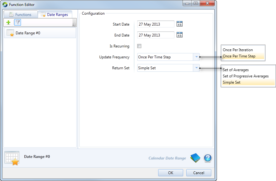
Figure 15. Function Editor (Date Range, period)
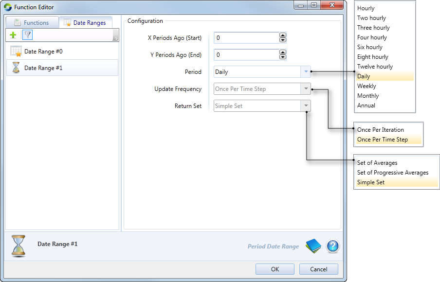
Figure 16. Function Editor (Date Range, time-step)
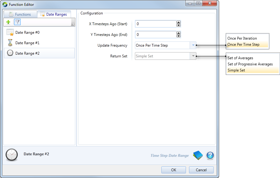
For all three custom calendar options:
- The Update Frequency popup menu offers a choice of OncePerTimeStep or OncePerIteration. The latter setting is only applicable to NetLP.
- The Return set popup menu controls the granularity of the returned result:
- If the range represents a single value, that value is returned regardless of this setting.
- Table 13 summarises what is returned if the range represents more than one value.
Table 13. Function Editor, Date Ranges (Variables)
| Option | Summary | Result |
|---|---|---|
| Simple Set | Returns the set of observations without modification | [1,2,3,4,5] |
| Set of Averages | Returns a set of the same size where each member is the average of all of the members of the set | [3,3,3,3,3] |
| Set of Progressive Averages | Returns a set of the same size where each member is the original value of that member averaged with the value of the first member. | [1,1.5,2,2.5,3] |
Where: input is the series [1,2,3,4,5]
Example
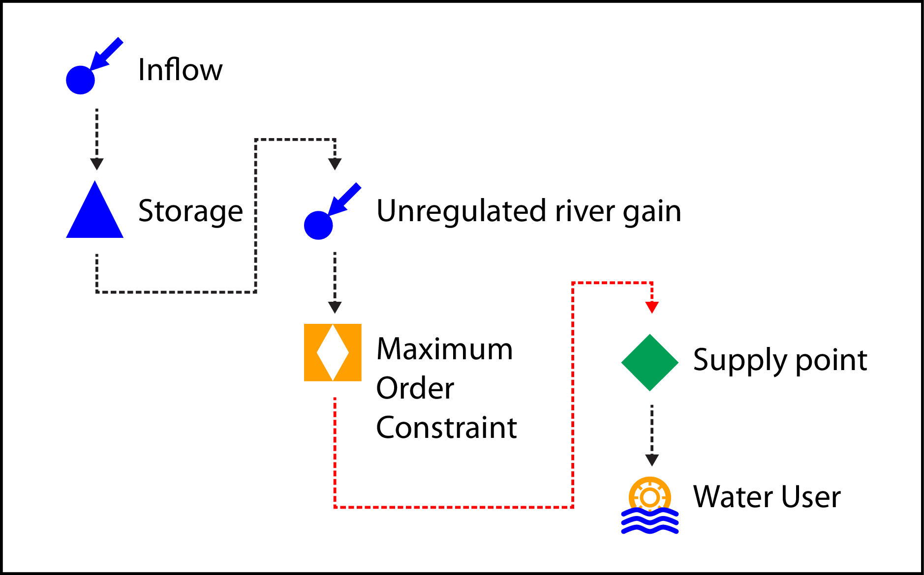
As an example, you can use a function or expression at a Maximum Order Constraint node to limit the maximum orders for each time-step. Assume that a channel constraint of 80 ML/day is required to prevent flows going overbank, except during floods (defined as more than 2,000 ML/day) when up to 3,000 ML/day is permitted as an environmental flow.
Figure 16 shows a fragment of the river network. Downstream demands are represented by a supply point and water user node. In the Function Editor, you specify the internal orders and unregulated river gain of the model using modelled variables. Maximum orders are then defined using an expression.
Figure 17. Maximum Order Constraint node (example)
In this case, the following components will be assigned:
- Storage 2: Requested flow rate - say, $Orders with a data range of Last time-step; and
- Inflow 3: Inflow - $predictedInflow, with the same data range as Storage 2.
Note that both variables will have ML/day as designated units.
Then, the following expression will return a value of 3,000 ML/day if flows are above 2,000 ML/day but 80 ML/day otherwise.
If(($predictedinflow+$orders) > 2000, 3000, 80
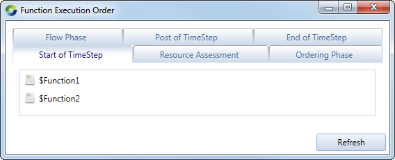
Debugging
- Recording - Recording is available for functions, pattern variables, and time series variables;
- Logging - The result of a function can be logged into the Log Reporter at a given day, by using the 'Add Log Date' context menu option for a function. This will output a log entry for each date specified. This output will include the result of the function, as well as all the functions and variables it uses at each time of evaluation; and
- Execution Order - The execution order can be viewed for each Time of Evaluation. Choose Tools » Function Execution Order to open this dialog.