Basic Concepts

Using Source is a two stage process. First models must be built, and then they can be used. Generally, these models can be classified into four categories, although there can be overlaps:

• River system models - these allow users to assess long-term impacts of water resource policy on system storages, flows and water shares, and develop better ways of managing river systems;
• River operations models - assist water authorities to optimise their day-to-day operations, such as water releases to meet irrigation demands and environmental requirements;
• Catchment models - provide information on the source, transport, transformation and fate of nutrients and pollutants. They are commonly used to develop, test and refine management strategies to improve water quality in rivers and reduce loads to receiving waters; and
• Urban models - allow the optimisation of urban supply systems and the development and refinement of water conservation strategies.

There are features common to all models which are described next. All models simulate flow; some models also simulate constituents.

Flow

Flow is the rate of water movement past a point per unit time. In Source, it refers to water moving through a node-link network (from sub-catchments, through links to an outlet). Source can be used to predict flow at defined points in a river network, operating down to daily time-steps and reporting at daily to monthly to decadal scales.

Constituents

A constituent is a material that is generated, transported and/or transformed within a catchment. Constituents commonly include sediments, nutrients, contaminants (eg pesticides, heavy metals), pathogens and other water quality properties. Constituent generation models govern the way constituents are generated within a Source model. This may be static or time-varying and could be a function of flow or other variables.

Representing systems in Source

A Source model is a simplification of the real world, and uses certain conventions to represent important characteristics of the system being simulated. Key features include:

• Catchments and sub-catchments - areas that generate runoff and constituent loads;
• Functional Units - areas within a sub-catchment that have similar behaviour in terms of runoff generation and/or nutrient generation. These could be, for example, areas with common land use;
• Nodes - points where flows and nutrients enter the river network, or where some process that is important for modelling, occurs (eg flow measurements at a stream gauge); and
• Links - used to join nodes and to store, route and process flow and constituents.

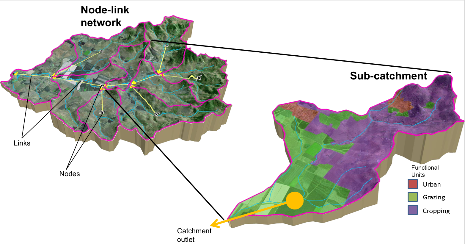
Source uses a node-link style modelling system for generating, transporting and transforming water and constituents within the major channels in a catchment (see Figure 1). Note that not all streams can be modelled, so you must decide which ones are important for a particular application. In urban applications, the basic Source features (nodes, links etc) can be used to create the functionality to model systems such desalination plants and storm water harvesting applications. Details are provided in the User Guide.

A catchment is the entire area of interest that is being modelled. The first step in modelling is to divide a catchment into sub-catchments. Sub-catchment boundaries can be determined based on stream topography and landforms calculated from a Digital Elevation Model (DEM), or through the analysis of topographic maps.

Catchment analysis is dealt with in detail in the Geographic Wizard for catchments, and the Spatial data pre-processor. Figure 2 shows an example of a node-link network, which is made up of several sub-catchments.

A selection of sub-catchments will determine the location of the nodes in the node-link model, so sub-catchments need to represent the major sources of water inflows and nutrient inputs. In Source, a sub-catchment is the area flowing into a node. There is no explicit representation of a stream network or surface routing within the sub-catchment.

About functional units

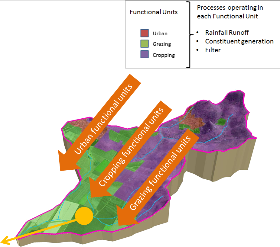
Sub-catchments are divided into areas with a common hydrologic response or behaviour called functional units (FUs), based on various combinations of land use or cover (eg forest, crop, urban), management, position in landscape (flat, hill slope, and ridge) and/or hazard (however defined). Figure 2 shows an example of this.

Three basic processes are defined to operate in a functional unit:

• runoff generation - several different rainfall runoff models are available in Source and include Simhyd, AWBM, and Sacramento. It is also possible to use an observed catchment surface runoff depth;
• constituent generation - produce materials or contaminants such as total suspended solids and total nitrogen; and
• filtering - represents any transformation or storage of constituents that takes place between when they are generated and when they reach a sub-catchment node. It allows representation of physical processes that may occur due to riparian buffers, small dams, detention ponds, or denitrification processes.

Each process is applied as a set of algorithms that deliver the resulting output to the sub-catchment node. The Scientific Reference Guide provides details on the models available for each.

A rainfall runoff model, a constituent generation model and a filter model can be chosen for each functional unit. In some scenarios, the different functional units will use the same component models - for example using the same rainfall runoff model across units but with different parameters that define different runoff attributes (eg. pervious area). There are also cases where models may need to be different for each functional unit. For example, to represent the differences in rainfall response in an irrigated agricultural field vs a native forest. Similarly, different constituent generation and filter models can be used in different FUs or different subcatchments. The combination of runoff generation, constituent generation and filtering produces the output for a particular functional unit. In some individual sub-catchments or in some Source applications, only one or two of these processes may be required.

The outputs from all the functional units within a sub-catchment are combined as inputs to the node for that sub-catchment. In this way, output is lumped at the sub-catchment scale.

Source also supports a split of flow and loads into notional surface (quick) and subsurface (slow) portions from each FU.

About nodes

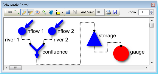
Nodes represent places where actions or measurements occur in a river system. For example water can be added, extracted, stored, recorded, or have a change in ownership. A node can be used to represent things that actually happen over a large physical area but which, for modelling purposes, occur at a single point, such as inflows from a catchment, or extractions from a group of off-takes. In sub-catchments, they provide a position in the catchment network where water management information, such as extractions and demands, can be placed. In Source, nodes are depicted using the icons shown in Figure 3.

Links represent river reaches but there are some important differences. A reach refers to a physical section of a river, while a link is a logical connection within a Source model. A link will sometimes be defined as having zero length (to conveniently represent certain processes), which is not possible for a reach. Links act to store water and route or process water and constituents passing between nodes (Figure 4). You can only connect nodes using links. You cannot connect two links to each other without an intervening node. Links also allow modelling of interaction with the floodplain.

In Source, links are depicted as lines with arrowheads indicating the direction of flow. Links allow modelling of several basic ‘processes’. Refer to Links for the different types of links available.

Model workflow

Source modelling comprises of the following four steps:

• Build;
• Calibrate;
• Run; and
• Report.

Building a model in Source is an iterative process. Once you start building it, you can collect more information, and refine the process and outputs, until ultimately the model is considered ‘fit for purpose’. Generally, a simple model is developed first, and this will continue to be refined for years as new questions or issues arise. The model you are developing now may be still be in use 20 years later, so it is important to be organised, systematic and to document all major decisions. Refer to Guidelines for Water Management Modelling.

The general approach to model building is as follows:

• Draw a schematic diagram representing the basic physical structure to be modelled. 

  Refer to Adding nodes to a model and Adding links to a model. Include the major waterways, stream gauges, inflows, diversions and outflows. You can begin the process of dividing a catchment into sub-catchments;

• Collect data on land use, flows, and other features that are important for your model. For a river system model you will need information on diversions and return flows. For a catchment model, you will need information on nutrient generation rates from different land uses. Urban models will have their own specific data requirements;
• Go back and refine the model schematic to take account of any new data that you have collected;
• Build the model in Source. This is referred to as populating the model because all parameters must be entered and their behaviour specified; and
• Calibrate the operational parameters. The purpose of calibration is to ensure the model is a reasonable representation of the current situation. It is important to be confident about this before testing the effect of any changes. Calibration will need to be revisited if the intended use of the model changes. To calibrate catchment models, refer to Calibration Wizard for catchments.

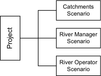
A Source model consists of two parts - a project and one or more scenarios. A scenario is the representation of a node-link network in Source. A package of scenarios is called a project. The relationship between a project and a scenario is shown in Figure 5.

A project is the wrapper for a collection of one or more scenarios. It identifies the project name, description, and any scenarios associated with the project. You can only have one project file open at a time and you should not open the same project file using more than one copy of Source.

A scenario describes the major processes in a river system or catchment that are modelled. This includes catchment and sub-catchment definition, rainfall runoff and constituent generation models, data sets and parameters. You can create multiple scenarios to:

• Break complex projects into distinct parts; or
• Duplicate existing scenarios to conduct what-if experiments without disrupting the original.

Any change to the definition of sub-catchments, node-link network, FUs, or the models within FUs, forms a new scenario. Similarly, a different set of inputs or parameters can be used to set up a new scenario, such as a change in land use or a climate change.

Time-steps

The following sections provide an overview of some important features in Source.

About time-steps and time-stamps

For clarity, the following definitions apply:

• Time-stamp - a date and an optional time on that date. A time-stamp represents a moment in time.
• Measurement - a value, for example, a flow measurement would typically have units for megalitres per day.
• Observation - a time-stamp plus at least one associated measurement.
• Time series - a file or database containing a set of observations in monotonically ascending order of time-stamp.
• Time-step - the resolution of the executing model. A time-step is a multiple of whole seconds and represents a duration of time, as distinct from a time-stamp which represents a moment in time.

Source uses the time-stamps in your time-series files to determine the time-step for the model. For example, if your time-series files contain daily time-stamps then Source operates on a daily time-step. For this reason, you need to ensure that all time-series files in a model use the same time-stamp granularity.

The number of seconds, or duration, of a time-step is calculated by subtracting the first second of the current time-step from the first second of the following time-step. When the model is operating in seconds, minutes, days, hours or weeks, the number of seconds in a time-step will always be fixed. For example, a day always contains 86,400 seconds (leap seconds are ignored). However, once time-step granularity reaches a month or more, the number of seconds in a time-step is variable. For example, the number of seconds in a month depends on whether the month contains 31 days; and for February and a whole year, whether the year is a leap year.

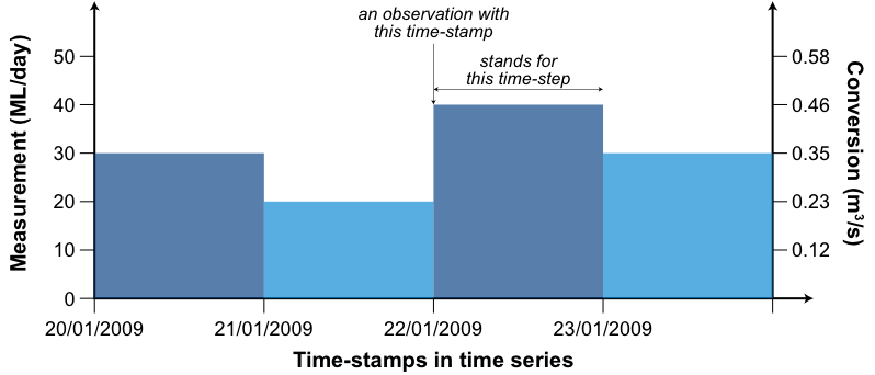
When reading a time series, Source assumes that the measurements in each observation were made at the first instant of the associated time-step, and that each measurement stands for the whole of the time-step. The measurements associated with time-stamps are expressed in units that you specify, either in the time series itself or in the feature editor when you load the time series. For example, a common unit would be megalitres per day. Regardless of the units of the original measurement, for internal use, Source converts each value to cubic metres per second using the number of seconds in the time-step.

Source does not interpolate between adjacent observations or otherwise attempt to calculate mean data or moving averages. The single value at the start of the time-step stands for the whole of the time-step.

Figure 6. Time-stamps vs time-steps

The relationships are summarised in Figure 6. Here, the time series of flows contains observations with daily time-stamps so Source adopts a daily time-step. The duration of each time-step is calculated as follows:

 

Equation 1

where all values are in seconds. An observation of 40 ML/day time-stamped 22/01/2009 is converted to 0.46 m³/s and that value stands for the whole of the time-step. Note that flows are always converted to m³/s for internal calculations but you can specify the units that are displayed.

It is up to you to ensure that your time-series files respect these assumptions.

Plugins and component models

They can either extend its user interface, or add steps or models to the Geographic Wizard.

Source supports a range of component models. These are mathematical models or algorithms that represent particular physical processes, such as rainfall runoff generation, flow routing or constituent filtering:

• Built-in component models. When you install Source, several component models are installed at the same time and some of these will automatically appear in the menus; others must be loaded manually;
• Component models, such as the River Harvesting Diversion Node model, that can be manually loaded into Source. A range of component models are available where specific user interfaces have been constructed; or
• Plugins are loaded into Source and run alongside a model. You can use these to process data from the output of a Source scenario. These component models are external to Source and must be compatible with the software .

All plugin models and tools listed in this guide have undergone quality assurance and testing procedures endorsed and supported by eWater Ltd. Any issues or problems that may occur with these plugins will be resolved by the Source software development team supported by eWater.

Third party plugins that are compatible with Source are available to download from http://www.toolkit.net.au. These plugins are externally developed through groups and organisations outside of the eWater Source Project and are not supported by eWater or the Source software development team. Using externally developed plugins for purposes outside of their intended use is not recommended or endorsed by eWater.

Instructions on writing a plugin for Source are available from /wiki/spaces/SC/pages/51643422.

Water balance

Water balance, or mass balance, determines whether a model has been calibrated properly, based on the principle that water mass is preserved in the river system. It ensures that losses do not exceed inflows. Source ensures that water balance is respected in flow calculations, and mass balance is respected for calculations involving constituents. Additionally, it has a mass balance reporting functionality, which is a feature that other models do not have.

Units

This section provides an overview of the units used in Source.

Internal measurement units

River system modelling typically focuses on the distribution, use and mass balance of water volumes within those systems. Accordingly, units for input data (eg time-series files) and results are commonly expressed in volumes per unit time-step for the model (eg. ML/day or GL/month).

In Source, regardless of the original units of the input flow data, the internal computational process is undertaken in cubic metres per second. All input data undergoes unit conversion using the number of seconds in the time-step. Source produces results (accessed via the Recording Manager) and data (for export) expressed in both user-specified units and in m³/s. The results are provided for completeness, so you are given the full picture of what the model:

• does with input data;
• uses to do internal calculations; and
• does to produce output data.

Units drop-down menu

Source provides several options for various units of measurements. A full list can be viewed using Tools » Unit Preferences..., as described in User preferences. 

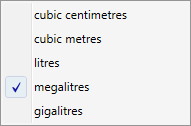
Figure 7 shows an example of volume data units (megalitres as the chosen unit) that are available in Source.