Cumulative Frequency Graphs

Cumulative frequency graphs present a plot of flow or concentration on the x-axis, against the frequency of occurrence of that value or lower on the y-axis. This may be thought of as the frequency of compliance with any given value. While time series graphs provide an overview of behaviour, cumulative frequency graphs provide a more informative summary of treatment performance.

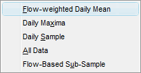
The Cumulative Frequency Graphs command on the Context-sensitive menu first presents a sub-menu of sampling regime options (similar to the Statistics sub-menu), as shown below:

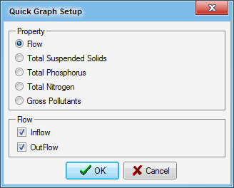
Clicking on any of the options opens the Quick Graph Setup dialog box (similar to the Time Series Graphs setup box), where the parameter of interest can be specified. The graph can be plotted for inflows and/or outflows, and the time-step can be specified, regardless of the time-step used to create the model. Cumulative frequency graphs can be plotted for flows and concentrations, but not for loads, so both lists contain fewer options than before.

The dialog is shown below.

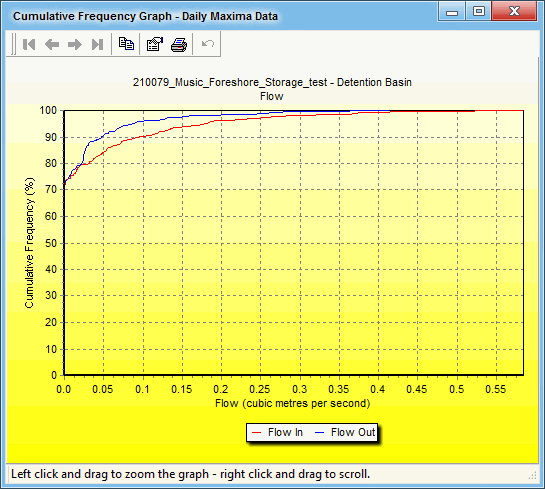
The cumulative frequency graph below shows inflow and outflow TSS concentrations for a pond treatment node downstream from another storage. There are substantial periods of zero flow, due to evaporation from this pond and further upstream. When flow is zero the concentration is undefined, leading to truncated curves of the form shown. The use of flow-based sub-samples in cases such as this is described in Flow Based Sub-Samples.

Properties of the graph can be modified using the edit button . Editable properties include colours, scales and displayed parameters. A graph can be moved, resized (within limits), and captured like any other window. It can also be copied to the clipboard () for pasting into other applications, or sent directly to a printer ().

Water quality standards will be displayed on the graph when they are active. They can be turned on or off using the check boxes on the Water Quality Standards definition box, accessed by the Water Quality Standards command on the Catchment menu. On a cumulative frequency graph, water quality standards take the form of a shaded exclusion zone bounded by the specified concentration and compliance frequency. A cumulative frequency curve that enters the shaded zone does not comply with that standard.

There are five sampling regime options for cumulative frequency graphs:

Flow-weighted Daily Mean cumulative frequency graphs are plotted from the flow-weighted daily mean data for flow and pollutant concentrations (the pollutant concentration is calculated by summing the load transported for the day, and dividing by the daily flow). This provides a summary of typical conditions within a day, and in doing so, smooths the effect of short-duration spikes in flow and/or pollutant concentration. The calculation is the same as in Music Version 1 - the command wording has been changed for greater clarity.

Daily Maxima cumulative frequency graphs are produced by extracting the maximum values for each parameter in each day, and plotting the resulting subset of data. This can be useful for purposes such as determining the magnitude and frequency of concentration spikes which occur within a receiving waterway.

Daily Sample cumulative frequency graphs are produced by taking a sample of one time-step from each day (similar to a field-sampling program). To avoid any possible effect of diurnal cycles, music Version 2.1 takes the sample at a random time on each day.

The Daily Sample graphs should be used with caution, because daily sampling may give an inaccurate impression of the effectiveness of any stormwater treatment measure which provides attenuation of flows.

Consider a wetland with a notional detention time of 48 hours. Routine daily sampling (as distinct from event-based sampling) is unlikely to catch a short storm event (say 30 minutes) at the inlet. But flows and pollutant concentrations will be elevated at the outlet for many hours after the event, and most likely will be sampled. Hence for many events the flows and concentrations at the outlet will appear to be larger than those at the inlet, contrary to the information derived from all of the data. The length of record to reliably average out this anomaly (by scoring a representative fraction of hits on the inflow peak) may be prohibitively large. Nevertheless, the daily sampling simulation closely approximates one form of sampling used in practice.

All Data cumulative frequency graphs are calculated from the entire dataset (i.e. all time-steps) at a node or link, including any time-steps in which there is no flow. The All Data cumulative frequency graphs are NOT flow-weighted.

The shape of the cumulative frequency curve depends on the selected time-step. A shorter simulation time-step leads to a wider range of simulated discharge or concentration, and a more sharply curved cumulative frequency curve. As a result, a shorter simulation time-step gives a lower discharge or concentration for a given frequency over most of the range of cumulative frequency.

Flow-Based Sub-Sample cumulative frequency graphs are calculated in the same way as the All Data graphs, except that they are derived using only the time-steps which have inflow to the treatment node or link (or outflow in the case of a source node) within a user-specified range. The flow-based sub-sample can also be used to calculate tables of statistics. Flow Based Sub-Samples describes how to specify the upper and lower flow thresholds, and how to interpret the results. This feature allows the separate analysis of baseflow and stormflow periods.