Insight: Objective optimisation
Introduction
Insight is eWater’s multiple-objective optimisation decision support framework. This framework allows for more efficient evaluation of planning options than the traditional manual trial and error approach that is often used. In other words, the main aim of Insight is to optimise decision rules for multiple objectives. The framework allows optimisation across single or multiple scenarios. The optimisation tool enables a more thorough examination of potential planning scenarios and the resulting trade-offs between desired outcomes.
Insight allows you to define which parameters (called decision variables) must be considered in the optimisation framework. Decisions variables can be thought of as management levers that can be pulled to affect the outcome. For example, you may be unsure of what the operating rules for a new desalination plant should be used to meet the objective of minimising cost, or what the optimal operating rules are for transferring water between storages to meet supply security objectives and minimising environmental impacts. By creating decision variables for these operating rules, the optimiser will try hundreds or thousands of different operating rules based on these decision variables and determine how the rules perform against a set of specified objectives.
Results of an optimisation run can be used as follows:
- Tradeoffs between competing objectives can be identified and a desirable balance between objectives can be discussed; or
- Management options which achieve the desired outcomes can be identified.
Decision variables
The goal of optimsation is to acheive a set of defined objectives based on decision variables that act as management levers. For example, the amount of water to release for environmental flows, the level of demand, or the amount of water to order from alternative supplies.
When deciding on decision variables, it is important to consider:
- What the key drivers are likely to be (relevance);
- Which parameter in the model represents the decision variable;
- The number of decision variables, and the consequence of multiple decision variables;
- Are they discrete or continuous (“real” numbers)?; and
- What are realistic ranges? Are there any constraints on the likely acceptable range for the decision variables?
Objectives
Mathematically known as objective functions, these can contain multiple parts, such as measure of cost, a measure of environmental impact and a measure of social costs. Examples of objective functions might include: minimising the operating cost of the system, minimising environmental impacts, or minimising time spent in water restrictions. In Insight, objective funcitons must be expressed as minimisation problems. Maximisation problems can be optimised by expressing the objective function as a negative.
When choosing objectives, it is important to consider:
- The number of objectives;
- The independence of the objectives;
- Sensitivity of those objective functions to decision variables;
- The value of the objectives to stakeholders; and
- The ability to use outputs from the model to calculate the required objective.
Working with Insight
All tasks undertaken to carry out an optimisation run (from creating a settings file to the actual run) can be completed using either the Insight interface or a command line. Results for an optimisation run can be viewed in the interface only. These are described in further detail in subsequent sections.
Ensure that the following pre-requisites are met prior to installing Insight:
- Latest version of Source. This must be correctly installed prior to running Insight;
- Microsoft .NET framework v4 (or higher); and
- Microsoft C++ 2010 x86 redistributable package.
Additionally, at a minimum, Insight requires the following to run an optimisation:
- A Source scenario containing decision variables and objectives expressed as Source functions;
- Access to the Source command line tool;
- An Insight settings file (containing the Source project location, objectives and decision variables);
- The number of generations; and
- The population size of each generation.
The decision variables and objectives must be defined in the Source project as functions. Insight can then run the Source model thousands of times, setting different values for the decision variable expressions and evaluating the corresponding objectives for every individual run.
This means that in order for a Source parameter to be included in an optimisation problem, that parameter needs to be defined using the Function manager in Source.
Launching Insight
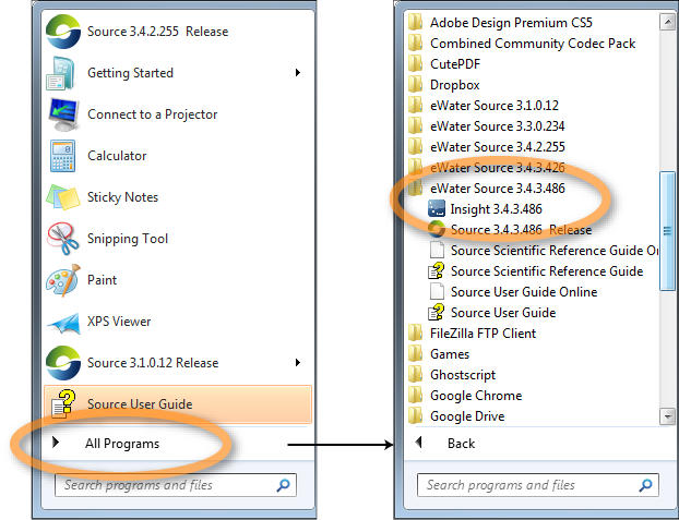
Figure 1 shows how to launch Insight once Source has been installed:
- Click on the Windows Start menu;
- Choose All Programs (shown on the left of Figure 1);
- Scroll down and click on the folder indicating the version of Source you have installed (In Figure 1, this is eWater Source 3.3.0.234); and
- Choose Insight from the list of programs listed (shown on the right of Figure 1).
Figure 1. Launching Insight
Using the Insight interface
When you open Insight for the first time, you may be prompted to point Insight to the location of the Source command line tool (RiverSystem.CommandLine.exe).
Figure 2 shows the user interface for Insight, which allows you to load Source projects, configure a settings file and perform an optimisation run.
The File menu items allow you to work with settings and results as follows:
- File » Load Settings - Load settings that were previously configured and saved (optional);
- File » Save Settings - Saves the current run settings;
- File » Load results - Loads the results of a previously saved optimisation run (optional);
- File » Save results - Save the results of the current optimisation run; and
- File » Exit - Quits Insight.
Figure 2. Insight user interface
Note: Prior to using Insight, ensure that all Source projects contain only one scenario.
Setting up an optimisation run/Creating a settings file
- Open Insight and click Browse (as shown in Figure 2) to choose the directory containing the project(s). Projects can also be in sub-directories below the directory pointed to. In Source (public version), you can only load a single scenario;
- Click Load to populate the left panel with all the available functions defined in the loaded projects;
- For each of the panels on the right, use the appropriate button to add or remove objectives functions or decision variables from the main function list to the individual panel. For example, click Add objective » to add an objective function to the Objectives panel. Moreover, to move a discrete decision variable back to the main list of objective functions, click « Remove discrete decision variable.
- In the Objectives panel, the Multi-project Aggregation Method drop-down menu allows you to choose how you want to process the objective function values passed from individual scenarios. By default Insight uses the final value of the specified function as the value of the objective function for each scenario. The Aggregate over full timeseries checkbox allows you to use the values of the objective function determined at each timestep, rather than just the last value (via the selected statistical function). You can also remove an objective from the Objectives panel by choosing it from the list and clicking « Remove objective. This will move the objective back to the main objectives list.
- Choose the number of generations and the population size of each generation. These parameters define how many simulation runs are performed by the optimiser. The required values will depend on the complexity of the optimisation project. If the number of runs is too small, the optimiser will not be given sufficient time to search for the multi-objective optimal set of results. The population size also sets the maximum number of points on the Pareto front or surface.
- Specify whether to run the optimisation on your local machine (enable the Run Source optimisation locally radio button), or across server endpoints (using the Run Source optimisation on endpoints radio button). Server endpoints allow you to run the optimisation across several machines simultaneously. Load the endpoints settings file by clicking Load Endpoints and point Insight to the appropriate file. If running Source optimisation on a local machine, set the number of cores to use with the Local server limit scroll button. The number of cores to use depends on the machine you are using.
- Save your settings using File » Save Settings. This creates a settings file, which can be used later.
The optimisation is now ready to be run.
Running an optimisation
Once you have nominated the location of Source, the Source project to optimise, and the objectives and decision variables, click Run to begin the optimisation.
On completion of the run, you will be prompted to save the results, which can then be viewed at a later stage if required.
Using the command line
Insight can be configured, set up (using a settings file) and run using the command line as well. This link shows some examples of how to use the command line for Insight. Note that an explanation of these commands is provided further down:
Creating the settings file
The settings file can be created in a text editor, such as Notepad, saved as a .txt file (such as Example_InsightSettings.txt) and must include the information shown in Table 1.
Table 1. Information required to create a settings file
| Information required | Example |
|---|---|
| Location of the Source project file | project C:\Insight\test\Example_project.rsproj |
| List of the objectives, using the global expressions in the Source project | ExportedOutput $reliabilityNeg ExportedOutput $unitcost ExportedOutput $Yieldneg |
| List of decision variables, using the global expressions in the Source project, along with their constraint | real $pipecapacity 0 200 |
Configuring the optimisation run
Once a settings file has been created, specify the following (as shown in Table 2) in the command line to configure the optimisation run.
Table 2. Information required to configure an optimisation run
| Information required | Example |
|---|---|
| Specify to run the Insight executable file | Insight.Optimiser.Console.exe |
| Location of Insight settings file | --configurationOption "C:\Insight\test\Example_InsightSettings.txt” |
| The number of cores / endpoints to use | --source 2 |
| The number of generations | --generations 6 |
| The population size | --population 100 |
| Output file name | --output “C:\Insight\test\Example_CommandLineResults_6x100.csv" |
Setting up server endpoints
Server endpoints allow you to run the optimisation across several machines simultaneously. It is recommended to discuss the use of endpoints with your IT department should you wish to choose this option.
If you wish to run the optimisation across multiple machines at once, you can do so using server endpoints, noting that:
- Each individual machine must have Source installed; and
- The project file will need to be located on a server where all machines can access it.
Endpoints can be set up manually or using the Powershell script. These are discussed separately next.
Manual set up of individual machines as endpoints
For each individual computer you wish to use in the optimisation, you will need to set it up as an endpoint(s). This is setup using the command line on each machine.
- Locate the IP address (type ipconfig in the command prompt) or machine name (in the Properties section of My Computer) for each computer you are going to use in the optimisation;
- In the command prompt, change the directory to the location of Source (ie. where Source in installed); and
- Setup the endpoint using the endpoint setup command. For example, in the following case, 8593 is the unique identifier for the endpoint:
RiverSystem.CommandLine.exe -m server -a net.tcp://localhost:8593/insight
Once setup is complete, a message will appear indicating this.
To use additional cores on an individual machine, you will need to set up multiple endpoints.
If you wish to open up another endpoint for the same machine, open up another command prompt, change to the Source directory, and enter a similar command, this time with a different endpoint identifier. For example:
RiverSystem.CommandLine.exe -m server -a net.tcp://localhost:8594/insight
Setting up endpoints using PowerShell script
You can also set up endpoints using the included PowerShell script.
Do the following on every machine that you wish to set up as an endpoint/s:
- Ensure that the RunSourceServersForInsight.ps1 file is in the same folder as RiverSystems.CommandLine.exe;
- Open PowerShell (Click on the Start menu (Windows 7), search for PowerShell, and press Enter);
- This method of setting up endpoints requires a change to the execution policy for each machine you wish to use as an endpoint. At the PowerShell command prompt, enter Set-ExecutionPolicy RemoteSigned. You will be asked to confirm the change (you can read more about this by selecting the relevant help topic). Choose Yes. Note that this needs to be done only once;
- Change the directory to the location of the RunSourceServersForInsight.ps1 file;
- Run the PowerShell script with ./RunSourceServersForInsight.ps1;
- The PowerShell script has automatically set up endpoints for you. Make a note of each endpoint, as these will be required when running the optimisation. Repeat this step across every machine that you wish to use as an endpoint. By default, the PowerShell script sets up two endpoints. To change the number of endpoints on the same computer, add the number of endpoints after the run command. For example: ./RunSourceServersForInsight.ps1 4 indicates 4 endpoints;
Finally, create an endpoints setting file using a text editor. Using the IP addresses or machine names (as located previously), specify the endpoints manually or via PowerShell. An example of such as file (Endpoints.txt) is shown below:
net.tcp://192.168.1.2:8593/insight
net.tcp://192.168.1.2:8594/insight
net.tcp://192.168.1.73:8595/insight
net.tcp://192.168.1.73:8596/insight
Running the optimisation
Once the settings file has been configured (along with endpoints if you are using them), set up the optimisation run itself.
Ensure that the parameters listed in Table 2 are entered. Then, press enter to begin the optimisation run.
As Insight computes the optimisation for each popluation, a completion notification is displayed in the command line.
Viewing optimisation results
To view the results of an optimisation run, choose File » Load results. This will load the Results dialog where you can view the results in various graphical formats.
Optimisation run results are compared to the Pareto Front. The Pareto Front is the set of solutions which have differing performance on each of the objectives. A solution is not on the Pareto Front if there is an alternative that is better on at-least one of the objectives but no worse on any objectives. In this case the solution is discarded as the alternative is clearly preferable. If the Pareto Front solutions are not changing, the optimiser may have satisfactorily completed its multi-objective search.
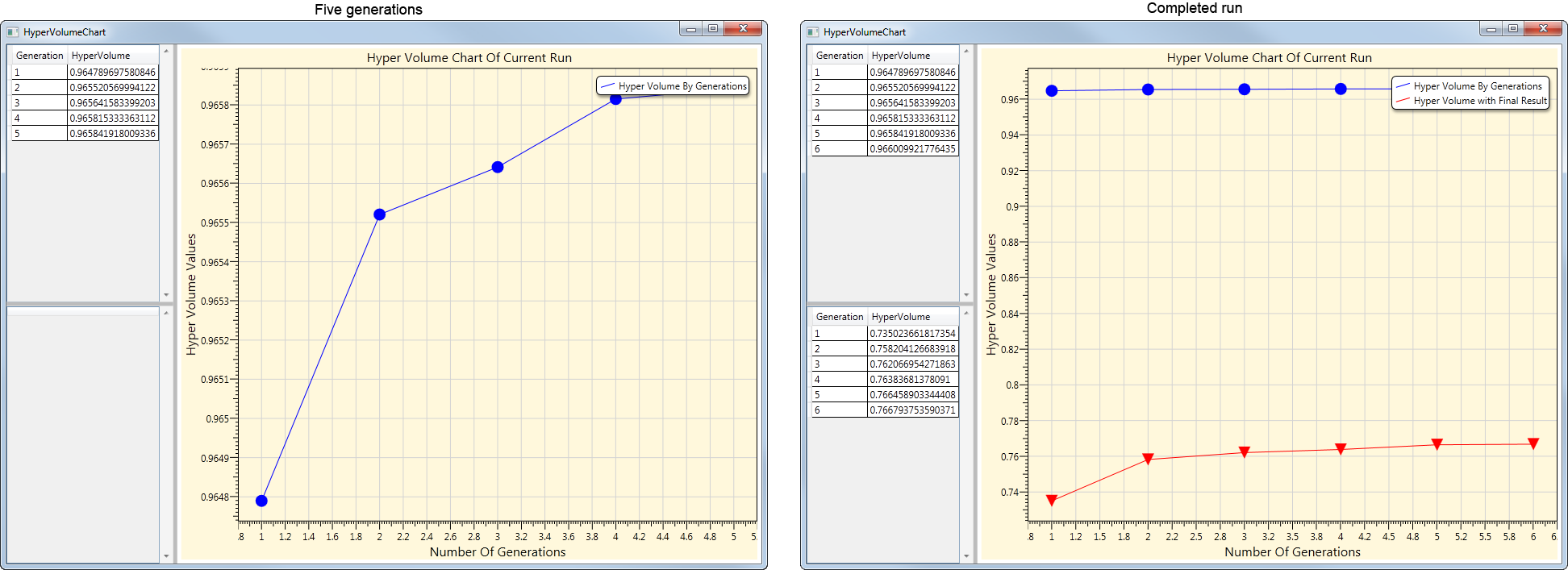
Hypervolume plot
During the optimisation run (when using the interface), after more than a generation is complete, you will be able to view the hypervolume plot – an indication of how the Pareto Front (selection of optimal results) is converging. The hypervolume provides an indication of the convergence of the model results towards the Pareto Front. The hypervolume is calculated based on the distance between a maximum non-optimal solution and the modelled results. In effect, the larger the hypervolume, the closer the results are towards reaching the Pareto optimal solution. The hypervolume provides an indication of the convergence of the model results towards the Pareto Front. It is calculated based on the distance between a maximum non-optimal solution and the modelled results. In effect, the larger the hypervolume, the closer the results are towards reaching the Pareto optimal solution.
Insight provides two plots of hypervolume when using the user interface (shown in Figure 3). The blue hypervolume plot is calculated whilst Insight is running, without knowing what the maximum non-optimal solution is (shown on the left of Figure 2). The red hypervolume plot is calculated at the end of the optimisation run, using the maximum non-optimal solution as reference. The hypervolume is a useful indication of how much the optimal solutions are changing – if the hypervolume plot is flattening out, this is a sign that more generations are unlikely to produce more optimal results.
Figure 3. Insight results, hypervolume plots
2D graph
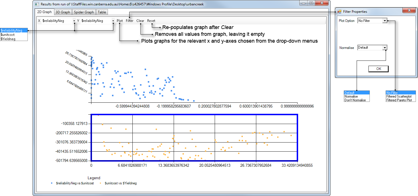
Click the 2D Graph tab at the top of the Results dialog to view two-dimensional scatterplots of the results (as shown in Figure 4). The drop-down menus for the x and y axes list all the objectives specified in the optimisation. To view the graph for a particular relationship, choose the relevant items from the drop-down menus and click Plot. The example shown in Figure 4 has three objectives defined: $reliabilityNeg, $unitcost and $Yieldneg. The points on the graph are forming the Pareto Front for this optimisation.
The Filter Properties dialog allows you to view the results in a specified range:
- Choose the type of plot (scattered or pareto) in the Plot Option drop-down menu;
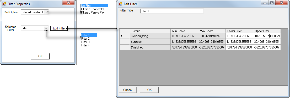
- In the Selected Filter drop-down menu, choose the filter and click Edit Filter;
- This opens the Edit Filter dialog (shown in Figure 4) showing the entire range of values.
- You can change the filter's name using the Filter Title panel.
- Edit any value by double clicking on the cell you wish to change and enter the required value (in the Lower Filter or Upper Filter columns); and
- Click OK to save changes close the Edit Filter dialog or Cancel to quit without saving.
Figure 4. Insight results, 2D graph
Figure 5. Insight results, Filter properties
3D graph
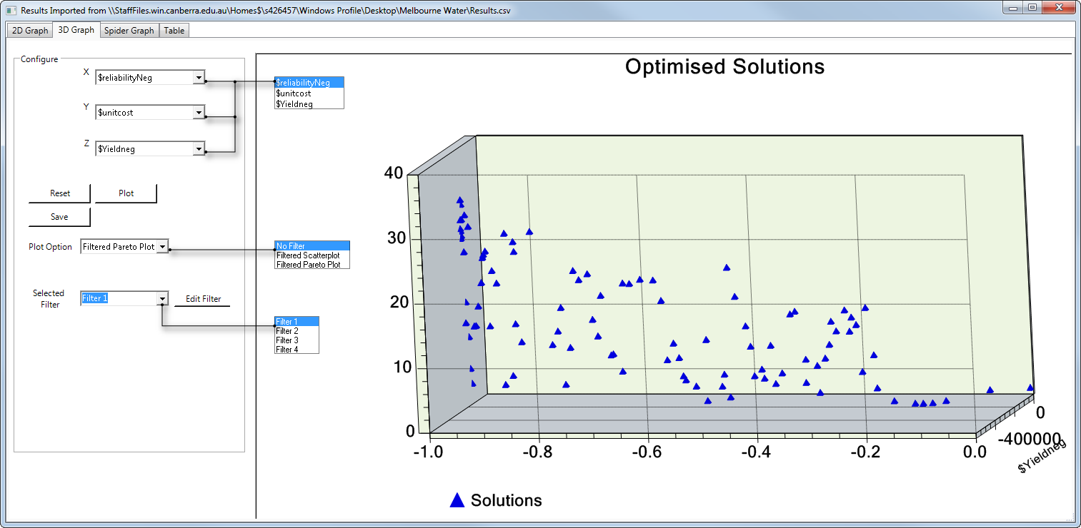
Click the 3D Graph tab to view a three-dimensional plot of the computed optimised solutions (shown in Figure 6). Just as with the two-dimensional graph, the individual solutions form a Pareto Front. The x, y and z-axes represent the objectives that were specified in the project. These can be changed using their corresponding drop down menus in the Configure panel on the left. Click Plot to change the axes; Reset to revert it back to its original state, and Save to save the results of the 3D graph to a file.
Additionally, you can filter the graph view to a specified range using the Filter Properties dialog (as shown in Figure 5) under the Plot Option drop-down menu.
You can also rotate the three-dimensional graph to make the results more meaningful, visually.:
- Press the Ctrl key on your keyboard and hold it down for the duration of the exercise;
- Right-click on the 3-D graph once;
- Right-click again and hold down the mouse button; and
- Move the mouse to rotate the entire graph.
Figure 6. Insight results, 3D graph
Spider graph
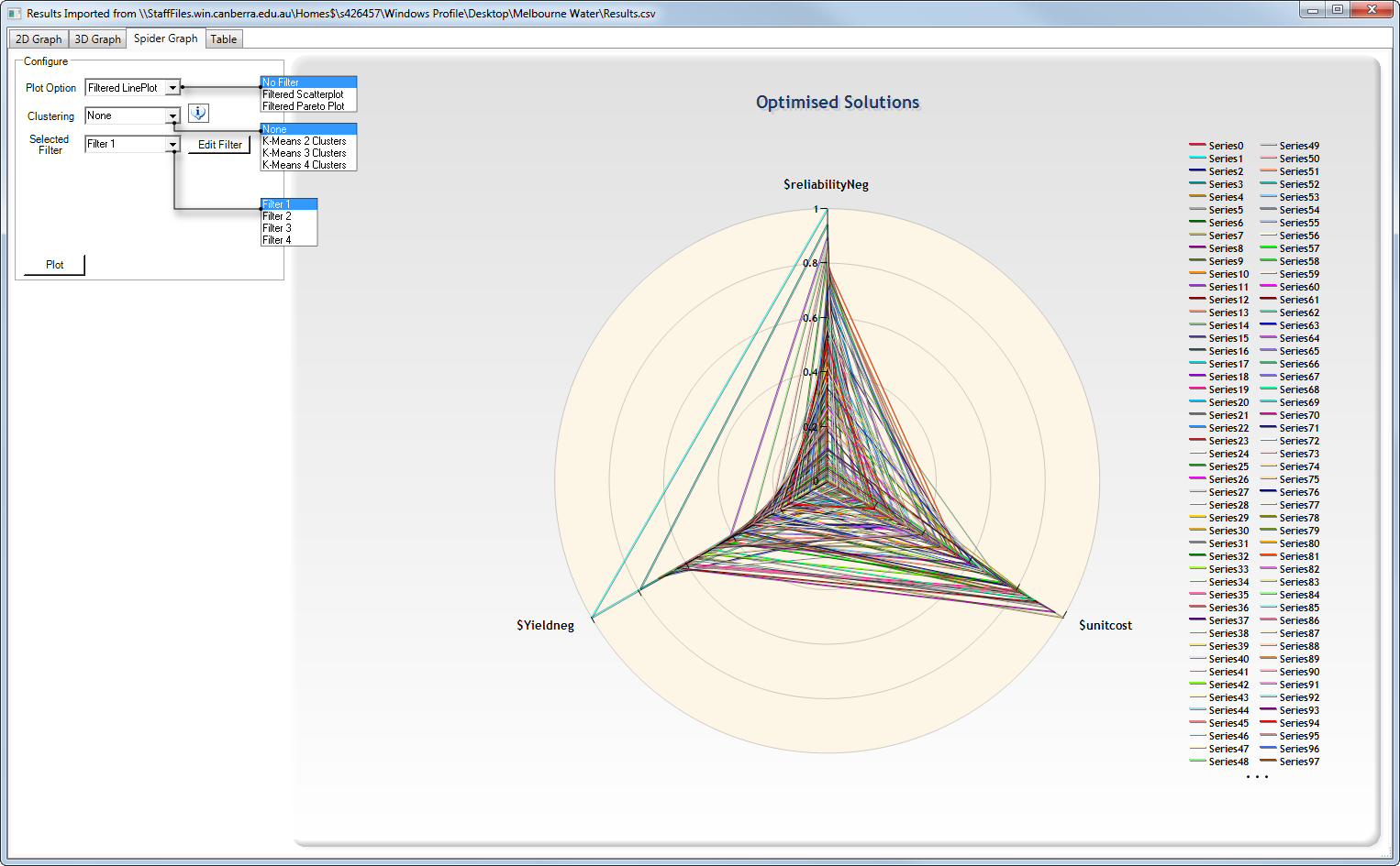
The third tab in the Results dialog shows the optimised results in a spider graph (as shown in Figure 7). You can use the Filter feature (as described previously) to view a filtered spider graph of the results.
Figure 7. Insight results, spider graph
Table
The final tab in the Results dialog shows all the results of the optimisation in a table. Figure 8 shows an example of the table, with all optimised solutions for each objective and decision variable specified in Insight. Note that the green arrow on the right allows you to save the decision variable to the Source project.
