Pride demand model
teamcity (Deactivated)
SysAdmin eWater
Analytics
The Pride demand model (developed for Victorian farming districts) replicates water requirements for a cropped area using a combination of climate data, crop culture and knowledge of traditional farming practices. These irrigation requirements are used to generate orders within regulated river systems or to drive extractions from unregulated systems. It is governed by factors which determine crop water use - principally the irrigation culture, climate, the characteristics of the soil and the type of irrigation system. In Source, a Pride demand model is configured and managed in the water user node feature editor.
To create a new Pride model, right click on Demand Models and choose Add Pride. The resulting window is shown in Figure 1. Parameters that must be configured are explained in Tables 1 and 2.
Figure 1. Pride demand model, main screen
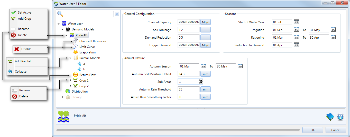
Table 1. Pride demand model, Configuration parameters
| Parameter | Description |
|---|---|
| General Configuration | |
| Channel capacity | Generally, this is the constraining capacity of the channel. If the capacity is not constraining, this figure should be very large (eg. 99999). |
| Soil drainage | This factor accounts for the fact that recorded deliveries to various irrigation districts (in terms of volumes of water per hectare) differed for the same crop types. This was thought to be due to the different soil drainage characteristics and access to groundwater. A default value of 1 should be used for the soil drainage factor, unless additional information is available (eg. measured data to calibrate the model). |
| Demand reduction | A close examination of actual delivery records indicated that by mid-April, some farmers begin to become reluctant to water their pasture into winter. This is mainly due to fear of water-logging should further rain occur and to avoid unnecessary labour and costs in irrigating. To simulate this reduction in demand, the user has the opportunity to apply a factor (the demand reduction ratio) to the estimated demand. A default factor of 0.5 should be applied, unless additional information is available. |
| Trigger demand | Due to the limited capacity of supply infrastructure, some irrigation managers apply rationing during peak periods to ensure the equitable distribution of water. Rationing capacities have been introduced into PRIDE to account for this practice. If you do not wish to ration demand, a very large number (eg. 99999) should be input here. This corresponds to the Rationing dates (as shown in Table 2). |
| Annual Pasture - The autumn irrigation of annual pasture is begun by application of an initial irrigation. Due largely to supply constraints, this volume of water cannot be delivered immediately to all annual pasture irrigators. Instead, the ‘starting’ of the annual pasture autumn season is staggered to cope with demand and infrastructure constraints. | |
| Autumn Soil Moisture Deficit | This parameter is used for an annual pasture only. A value of 14.3 is commonly used. If the autumn watering irrigation demand spikes unusually (particularly when compared to metered data), this value may be set too high. |
| Sub Areas | The autumn irrigation of annual pasture is begun by application of an initial irrigation. Due largely to supply constraints, this volume of water cannot be delivered immediately to all annual pasture irrigators. Instead the ‘starting’ of the annual pasture autumn season is staggered to cope with demand and infrastructure constraints. A new subarea is added daily until all areas are being irrigated. The default number of sub-areas is 6. |
| Autumn Rain Threshold | Threshold value for autumn rainfall that, when exceeded, triggers the start of irrigation. |
| Active Rain Smoothing Factor | The smoothing factor applied to average rainfall to calculate active rainfall for autumn watering of annual pasture |
The PRIDE model is set up to calculate crop water requirements by water year (Jul to Jun). You can specify the start and/or end dates of the irrigation season, autumn irrigation, rationing and reduction in demand. The default values (Table 2) should be used, unless additional information specific to the region, or if measured data that can be used to calibrate the model, is available
Table 2. Pride demand model, Configuring Seasons
| Parameter | Default dates |
|---|---|
| Start of Water Year | 1-Jul |
| Irrigation | 1-Mar to 31-May |
| Rationing | 15-Mar to 30-Apr |
| Reduction in Demand | 15-Apr |
Channel Efficiencies
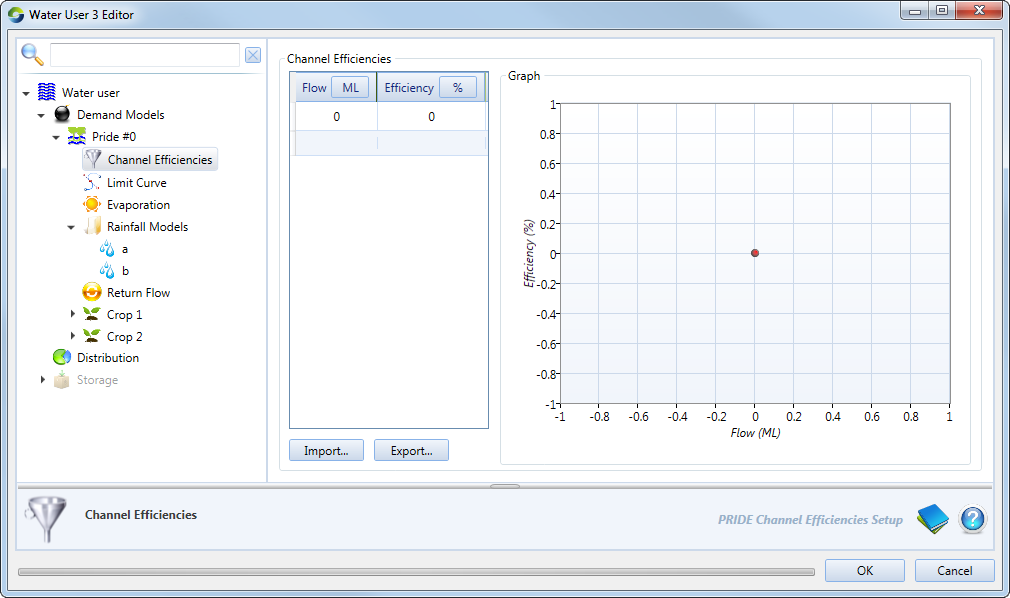
Here, you define the efficiency of the supply channel for a range of flows.
Figure 2. Pride demand mode, Channel Efficiencies
Limit Curve
A detailed description of the calculation and implementation of Limit Curves can be found in the Source Scientific Reference Guide.
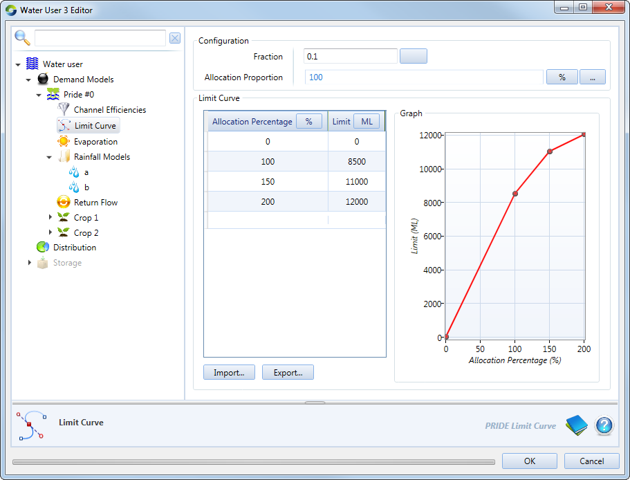
The limit curve prevents a demand node from using all of its available allocation too early in the season. It is defined based on a relationship between the announced or available allocation and limit. The Allocation Proportion can be set up as a constant or it can be customised using a function to vary according to the allocation percent set up in a Resource Assessment. Figure 3 shows an example where a constant has been specified for the Allocation Proportion.
The fraction represents a proportion (0 – 1) which determines the coefficients a, b and c of the limit curve equation. Please see the Source Scientific Reference Guide for more details on how ‘Fraction’ is implemented.
Figure 3. Pride demand model, Limit curve
The limit curve (Cumulative Restricted Demand in the results) will reflect the changes in Percent Per Share Entitlement (as shown on the left and right of Figure 4).
Figure 4. Pride demand model, Limit curve results

Evaporation
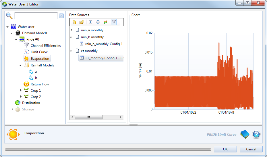
Evaporation is one of the climatic factors influencing demand and is specified using a time series. Figure 5 shows an example of the time series allocated to the model.
Figure 5. Pride demand model, Evaporation
Rainfall
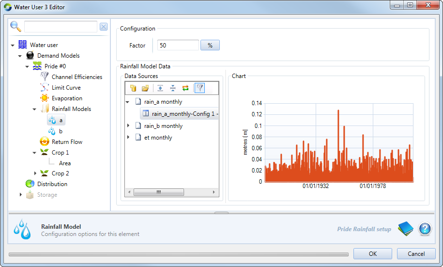
The second climatic factor affecting the model is rainfall. You can add rainfall models by right clicking on Rainfall Models and choosing Add Rainfall in the contextual menu. You must also allocate the weighting to assign to each rainfall model (shown in Figure 6), which must add to 1. Figure 7 shows an example of a rainfall model.
Figure 6. Pride demand model, Rainfall
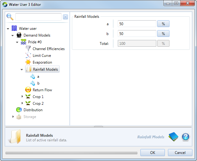
Figure 7. Pride demand model, Rainfall model a
Return Flow
Refer to Return flows for more information. Note that the percentage of volume supplied can be greater than 100%. This indicates that there is more return flow from the irrigator than diversions due to rainfall runoff.
Crop
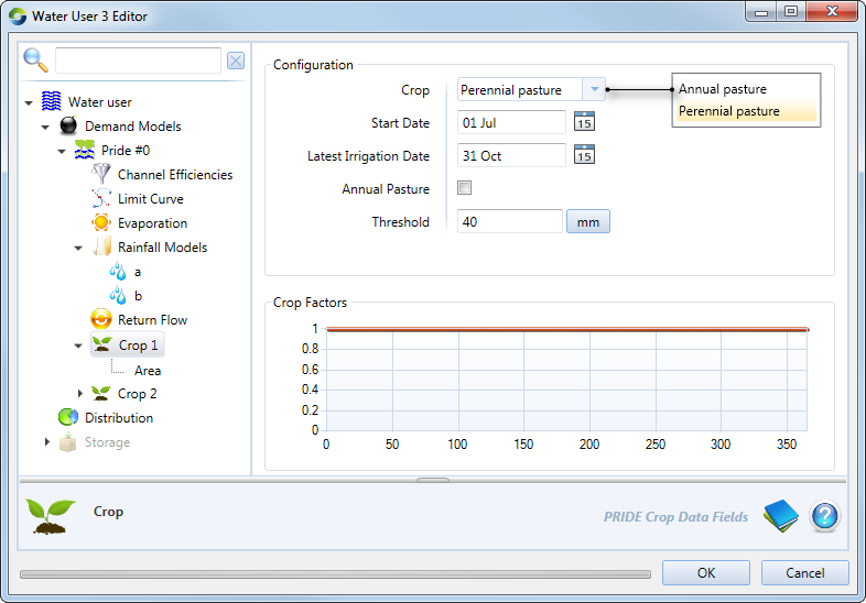
As shown in Figure 8, you can configure the following crop parameters:
- Crop - This can be specified as an annual pasture or a perennial one.
- Annual pasture - Allows you to setup a crop as annual pasture, which is traditionally irrigated in early spring and then again in Autumn.
- Threshold - irrigation at the beginning of the season is triggered when this threshold is exceeded.
Figure 8. Pride demand model, Crop
Crop Area
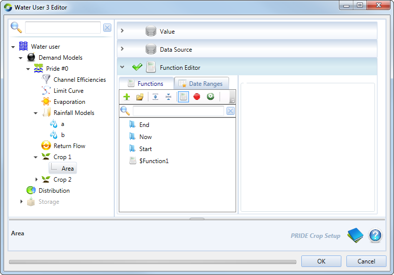
This can be specified as a single, constant value, a time series or as a function.
If an annual time series of crop areas is not used, you can specify a single set of crop areas, which applies to the entire model period. Ensure that the order and number of crops are consistent across all steps of model development. The model assumes that the first crop is Annual Pasture. If you do not wish to model Annual Pasture, then you must enter zero hectares of Annual Pasture as the first crop.
Note: If crop areas are small, your irrigation water requirements will be less and demand may be rounded to zero.
Figure 9. Pride demand model, Crop, Area
